Towards Machine Learning
Autoencoder
-
花式解释AutoEncoder与VAE - Sherlock的文章 - 知乎: 其实AE或者VAE的隐藏层(embedding layer)就是从input中提取出的精华特征,所以autoencoder也可以作为dimensionality reduction的方法(类似PCA)。
-
为什么Autoencoder可以用来做神经网络的预训练?AutoEncoder: 堆栈自动编码器 Stacked_AutoEncoder - LitoNeo的文章 - 知乎:但是有了batch normalization之后,是否还有预训练的必要?
https://github.com/kstoreyf/anomalies-GAN-HSC
ResNet
Skewness
CS 231n: Convolutional Neural Networks for Visual Recognition
- Syllabus
-
PixelCNN: could complete the data (Bach’s music). Neural density estimation could also generate fake video/voice/images.
-
https://towardsdatascience.com/auto-regressive-generative-models-pixelrnn-pixelcnn-32d192911173
-
https://google.github.io/tacotron/
-
Lecture2:
- Linear Classifier only learns one template for one category (the row of the weight matrix).
-
Lecture3:
- If the image changes a little bit, SVM loss (hinge loss) will not change.
- You can design your loss function based on how bad you think negative classifications are (linear hinge or squar ed hinge loss).
- Add an additional term in the loss function as regularization. L1 regularization prefers sparse solutions.
- Softmax loss (cross-entropy loss): - log probability = - log (normalize(exp(score_of_true_class))). Softmax loss is sensitive to a little change in the input image (thus the score). Actually
softmaxis a squashing function that turns scores into probability, then cross-entropy loss is used. - In DL, you always use analytic gradient (instead of numeric gradient).
- Getting learning rate correct is the first step in tuning hyper-parameters.
- Vanilla gradient descent, stochastic gradient descent (SGD), ADAM
- If we take the whole training set to calculate the loss, gradient, and update parameters, it will take a very long time to iterate over all images. We use stochastic gradient descent (SGD) and minibatch. For each time, we sample a small subset of the training set (called minibatch), and update the parameters based on these images.
- Feature representation:
- Extract some features of your images, then flatten features into a 1-D array, and feed it into linear classifier.
- Histogram of Oriented Gradients (HoG): detecting edge is critical to human vision system.
- “Visual words”
- Classical image classification methods first extract features and concatenate features together and feed them to a linear classifier. The feature extraction module will not get updated during training. NN is different, it gets updated during training.
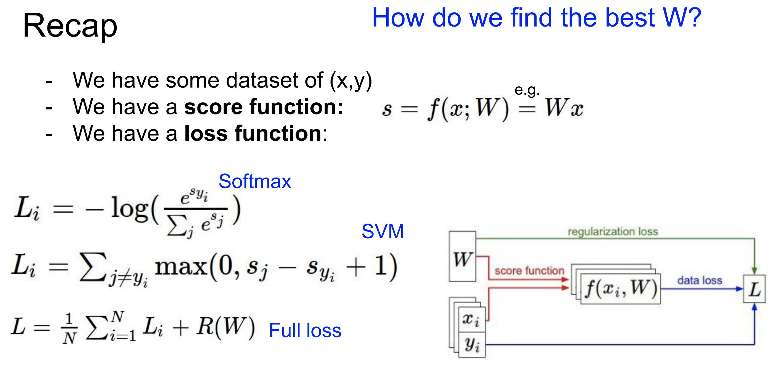
- Loss and regularization
-
Lecture4:
- Sigmoid: \(\frac{1}{1+e^{-x}}\)
- The gradient with respect to a variable should have the same shape as the variable (vectorized operations)
- Each row of the weight matrix is like a map: where to look for features
- more neurons = more capacity
- Actually three FC layers are just like \(f = W_3 \cdot \max(W_2 \cdot \max(W_1\cdot x))\). The notion of “layer” allows us to use efficient vectorized code (matrix multiplies).
-
Lecture5:
- CNN can also be used for object detection and segmentation.
- Activation map: the output of a convolution layer (and after activated by some function)
- In CNN, each filter looks for one type of feature. We use multiple filters/kernels.
- Filters at the earlier/later layers usually represent low-level/high lever feature. Each filter does convolution in 3 colors (rgb). The depth of output is the number of filters you have.
- Output size = (N + 2 * padding - F) / stride + 1 The number of filters is often powers of 2: 32, 64, 128.
- Pooling layer: make representations smaller and more manageable, i.e., direct downsampling. We only do pooling spatially, not in the depth direction. Common one is max pooling.
- FC: aggregate all features (identified by each Conv layer) and get a score for each category
- Architecture: [(CONV-RELU) * N – POOL?] * M – (FC–RELU) * K – SOFTMAX. N up to 5, M is large, 0 <= K <= 2.
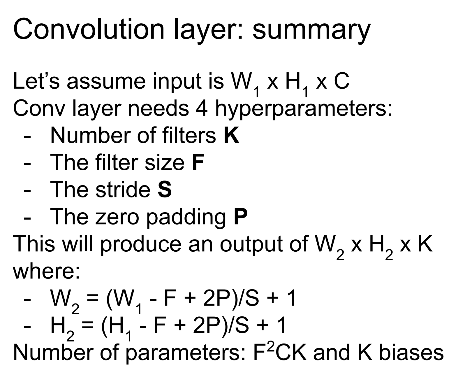
- CNN output size formulae
-
Lecture 6:
-
Activation functions:
-
Sigmoid: “kill” gradients when $$ x \gg 1$$ (i.e., gradients go to almost zero, called “saturated”); output is not zero-centered (check the video about this). - ReLU (rectified linear unit): doesn’t saturate, computational efficient, converge faster, biologically reasonable. Not zero-centered, saturated in negative x.
- Leaky ReLU: \(f(x) = \max(0.01 x, x)\), behaves very well.
- Maxout: \(f(x) = \max(w_1^T x + b_1, w_2^T x + b_2)\).
- TL;DR: use ReLU (careful about learning rate); try Leaky ReLU/Maxout/ELU; don’t use Sigmoid.
-
-
Preprocess data: do this before feeding data into CNN
- Zero-center (
-= np.mean(X)) + normalize (/= np.std(X)) - With images, we typically don’t do PCA and whitening.
- Subtract the mean image ([32, 32, 3] array) or per-channel mean (mean along each channel = 3 numbers)
- An important point to make about the preprocessing is that any preprocessing statistics (e.g. the data mean) must only be computed on the training data, and then applied to the validation / test data. E.g. computing the mean and subtracting it from every image across the entire dataset and then splitting the data into train/val/test splits would be a mistake. Instead, the mean must be computed only over the training data and then subtracted equally from all splits (train/val/test).
- Zero-center (
-
Weight initialization (still an active field in DL)
- Don’t set weights with equal values. Because if every neuron in the network computes the same output, then they will also all compute the same gradients during backpropagation and undergo the exact same parameter updates
- Don’t initialize with small numbers. a Neural Network layer that has very small weights will during backpropagation compute very small gradients on its data (since this gradient is proportional to the value of the weights).
- Xavier Initialization:
W = np.random.randn(fan_in, fan_out) / np.sqrt(fan_in), i.e., a Gaussian centered at 0 with \(\sigma = 1/\sqrt{N_{in}}\). See here for the derivation. - Sparse initialization: see the weights of most neurons to zero, but have several neurons randomly connected (with Gaussian weights).
- Bias initialization: typically set to zero.
- The current recommendation is to use ReLU units and use the
w = np.random.randn(n) * sqrt(2.0/n)
-
-
Batch normalization can be interpreted as doing preprocessing at every layer of the network, but integrated into the network itself in a differentiable manner.
-
For each FC layer (before activation ReLU), we normalize the data on a mini-batch level: subtract the mini-batch mean and divide by the mini-batch std. This is a differentiable function, hence able to backprop.
\[\widehat{x}^{(k)}=\frac{x^{(k)}-\mathrm{E}\left[x^{(k)}\right]}{\sqrt{\operatorname{Var}\left[x^{(k)}\right]}}\]
-
-
A Short Introduction to Entropy, Cross-Entropy and KL-Divergence
- Entropy: \(H(p) = -\sum_{i}p_i\log(p_i)\), the average information we get from the true distribution.
- Cross-entropy between two distributions (also a “distance” between two vectors): \(H(p,q) = -\sum_i p_i \log(q_i)\), the average information we get from the assumed distirbution.
-
Kullback-Leibler divergence: $$ D_{KL}(p q) = H(p,q) - H(p) = \sum_i p_i \log\left(\frac{p_i}{q_i}\right) $$. - Softmax loss: to minimize the distance between the true probability distribution and the estimated distribution. For image classification task, the loss becomes \(-\log q_{\text{true}}\).
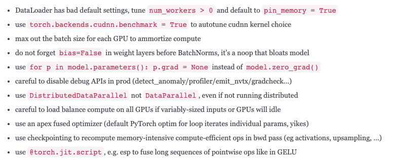
PyTorch Performance Tuning Guide - Szymon Migacz, NVIDIA
- Optimizing PyTorch code
The State of Machine Learning Frameworks in 2019
- “Researchers are abandoning TensorFlow and flocking to PyTorch in droves. Meanwhile in industry, Tensorflow is currently the platform of choice, but that may not be true for long.”
- PyTorch for researchers: simple, great API (pythonic), nice performance.
- Industry is slower to adopt new technologies than researchers. Researches care about fast iteration, easy-to-use on their own machine. But industry cares about performance (1% faster means a lot to them), ability to transfer to mobile devices, etc. TensorFlow has solutions for all these issues.
Deep Learning with Structured Data
- Chap 1
- Drawbacks of DL: large data volume (slow); non-transparent algorithm (well-known); tuning lots of things (overfitting, exploding gradients, and other hyperparameters).
- Solutions: transfer learning (use a well-trained model as the startpoint for another task); use commercial cloud platforms
- Structured data (tabular): relational database (rows and columns in a table), SQL. Unstructured data: image, video, audio, also text from HTML/XML/JSON. Many of the celebrated applications of deep learning have been with unstructured data such as images, audio, and text.
Gaussian Process in Machine Learning
Deep learning and Astrophysics
Finding Strong Gravitational Lenses in the DESI DECam Legacy Survey
Cluster finder (Song)
Another interesting application of deep learning would be cluster finder. I just know that someone is working on it, but have not seen a paper. There is a very short talk at the LSST-UK meeting now: https://lsst-uk.atlassian.net/wiki/download/attachments/650412049/Using_deep_learning_to_search_for_galaxy_clusters.pdf. The idea is pretty straightforward, given a training sample of galaxy clusters down to certain richness/halo mass, is there a network that can select all the clusters in another dataset? Or even better, if the training sample comes with labels like redshift and richness, can the network predict that? This would be a much, much more interesting application…but also it will be much more complicated. Anyway, just another random idea I’d like to write down before I forget…
The use of convolutional neural networks for modelling large optically-selected strong galaxy-lens samples
Photometric redshifts from SDSS images using a Convolutional Neural Network
The use of convolutional neural networks for modelling large optically-selected strong galaxy-lens samples
Tidal Features at $0.05 < z < 0.45$ in the Hyper Suprime-Cam Subaru Strategic Program: Properties and Formation Channels
- Her talk on her paper: Characterizing Tidal Features Across the Mass Scale with HSC