astro-ph Reading in 2019

Feel very ashamed for the decadence in the past year 2018. I will try to read as many paper as possible and do my best in 2019.

AAS-Nova

Astrobite

December 2019

Luis’s tips on writing paper

I am so tired of correcting grammatical and typographical mistakes that I will write a memo.

Proper use of $\sim$ vs. $\approx$. The former is used when referring to an approximate value of a number, but in a sentence when it is not preceded by a variable, as in “by a factor of $\sim 2$”. The latter is used when the value is preceded by a variable, as in “scale of $r \approx 2$”. Never use “$r \sim 2$”. Similarly, the following syntax is wrong, and looks silly: “redshift “redshift $2 \sim 3$”. It should be “redshift $\sim 2-3$”
There should be a space between a value and its units, such as $1\,\sigma$ $10\, M_\odot$
Use exponential notation, as in km~s$^{-1}$ instead of km/s
All negative signs should be in mathmode, $-$
Don’t use negative angles for position angles; for the equivalent positive angle, add 180 degrees
for fractional values of arcseconds, use 2\farcs5 instead of 2.5\arcsec
“e.g.” is usually followed by a comma
except in extraordinary circumstances, citations should be listed according to year of publication, in alphanumerical order.
Understand notation for specifying ionization states of ions. It is H II, not HII; H I, not HII; H_2, not H2; [C II], not [CII].
The word “data” is plural.
“these data, which are perfect”; “these data that went into the analysis”. Note the placement of comma before “which”
“rather than” is not proper English; should be “instead of”
Space satellites should be give in italics, as in {\it Spitzer}.
Subscripts with single letter should be in italics, as in r_e, except when it refers to a proper noun, as in r_E, where E may refer to Eddington, or to a bandpass, such as m_B, A_V, etc. Subscripts with more one letter should be in Roman fonts, as in r_{\rm eff}.
Proper align the columns in your tables
All fonts used in figure labels should be identical to those used in the main text. Same applies to tables.
logX should be log X
It is much easier to refer to multiple panel figures when they are labelled with (a), (b), etc.
References to papers on Astroph should be accompanied by a full reference if available, as in xxxx, et al. (2019), ApJ, in press (arXiv: xxx.xxx)
Do not list the bloody DOI numbers.
I hate the biblio feature, because half the time I cannot compile it on my MAC. It also makes the text manuscript horrible to read, because I have no idea what the encrypted reference refers to. But I will not insist on this. I just don’t understand why on Earth anyone thinks it’s a good idea.
Run spell check. Proof read. If still not sure, ask someone to help you. Then proof read again. My time is too valuable to be your secretary.

I can go on and on, but I’ll stop for now. Please pay attention to these details in your manuscripts. Since at any one time I have 5-10 manuscripts in my inbox, my response time will be significantly slower if I am annoyed by what you send me.

Luis

Forecasting: Principles and Practice

Reproducible science/research

Some good points here: You hear this statement a lot from many scientists: “software is not my specialty, I am not a software engineer, so the quality of my code/processing doesn’t matter. Why should I master good coding style (or release my code), when I am hired to do Astronomy/Biology?”. This is akin to a French scientist saying that “English is not my language, I am not Shakespeare. So the quality of my English writing doesn’t matter. Why should I master good English style, when I am hired to do Astronomy/Biology?”

Estimating Sky Level

NoiseChisel: NOISE-BASED DETECTION AND SEGMENTATION OF NEBULOUS OBJECTS

Gravitational Wave step-by-step

TOPCAT and how to use it for Gaia

Hybrid Physical-Deep Learning Model for Astronomical Inverse Problems

11/11/19 - 11/17/19

Learning to speak fluently in a foreign language: Multilingual speech synthesis and cross-language voice cloning

DESC LSST school

Double slit experiment using quasar?? http://news.mit.edu/2017/loophole-bells-inequality-starlight-0207, http://news.mit.edu/2018/light-ancient-quasars-helps-confirm-quantum-entanglement-0820

文献计量：https://bibliometric.com/results.html

Web of science: https://apps.webofknowledge.com/?Init=Yes&SrcApp=CR&SID=6Fd8SyBh3A3wR4zYh87

11/04/19 - 11/11/19

Astro2020 Science White Paper: Empirically Constraining Galaxy Evolution

Proposed by Peter Behroozi. Empirical relations are very important in understanding galaxy formation and evolution, by combining simulation and observations. Empirical relations can be applied in simulating mock catalogs (for survey designs) and provide feedback of simulations.
Empirical relations of galaxy - halo connection is well-established. However, more empirical relations can be done in multiple areas: how galaxy star formation history, morphology, gas content, SMBH mass, SNe/GRB/FRB rate depend on basic properties of galaxy/halo/environment/redshift.

Astro2020 Science White Paper: The Local Relics of of Supermassive Black Hole Seeds

Proposed by Jenny Greene. We have discovered stellar-mass BH, SMBH, but no solid evidence of intermediate-mass BH has been found. LIGO contributes to our understanding of BH mass function. But now, how high-z massive quasar formed? Where is IMBH? We don’t know. But with next-generation ground-based telescope, we will be able to tackle this problem. IMBH is expected to be residing in GCs and dwarf galaxies (low-mass, pristine of BH seeds). However, recoil effect could blow out IMBHs out of GC.
Astrometrical approach: observe stars in a GC, determine the astrometry motion of each star and diagnose potential IMBHs. This requires better than 10 mas astrometry precision, which could be achieved by 30-m telescopes with the help of adaptive-optics.
IFU approach: it’s possible to observe the velocity dispersion around IMBH using IFU mounted on 30-m telescopes. This requires 15 - 20 km/s resolution (R=8000) in spectroscopy to detect 10000 solar mass BHs.
On the other side, synergy among 30-m telescopes and next-generation GW detectors (LISA) making the detection of IMBH more possible.

Planck evidence for a closed Universe and a possible crisis for cosmology

Broadband Intensity Tomography: Spectral Tagging of the Cosmic UV Background

The Sloan Digital Sky Survey extended Point Spread Functions

10/14/19 - 10/20/19

Milgrom: MOND vs. dark matter in light of historical parallels

Shany: A Tip of the Red Giant Branch Distance to the Dark Matter Deficient Galaxy NGC 1052-DF4 from Deep Hubble Space Telescope Data

10/07/19 - 10/13/19

Nearly all Massive Quiescent Disk Galaxies have a Surprisingly Large Atomic Gas Reservoir

The Two LIGO/Virgo Binary Black Hole Mergers on 2019 August 28 Were Not Strongly Lensed

The LIGO/Virgo gravitational wave events S190828j and S190828l were detected only 21 minutes apart, from nearby regions of sky, and with the same source classifications (binary black hole mergers). However, the large separation is much more consistent with two independent, unrelated events that occurred close in time by chance. S190828j and S190828l were probably not lensed images of the same merger.

A PSF-based Approach to TESS High quality data Of Stellar clusters (PATHOS) – I. Search for exoplanets and variable stars in the field of 47 Tuc

How to convert an image from TESS to the light curve? Precise photometry is crucial for discovering exoplanets. This paper harnessed a PSF-based method which is alike our MRF. They calculate (stack) a PSF and then interpolate it for a given position. Then surrounding stars will be subtracted using that PSF and GAIA magnitudes, leaving the target star. At last a PSF-photometry will be applied to that star. Overall they find good consistence with existing methods and find a new exoplanet candidates in a GC called 47 Tuc (famous for amateur.)

PSF stacking: Anderson J., Bedin L. R., Piotto G., Yadav R. S., Bellini A., 2006,

Seeing Cosmology Grow

Peebles!!! Peebles!!! Peebles!!!

The Globular Cluster Population of NGC 1052-DF2: Evidence for Rotation

Main points against Pieter’s paper: 1. Wrong distance (should be 10 Mpc); 2. Wrong statistical approach when calculating the velocity dispersion.

The mass estimation relies on the assumption: relaxed and pressure supported. The estimation of dynamical mass would change if GCs are dominated by a global rotation. The author employed a toy rotation model into the Bayesian statistics. They find that the amplitude of rotation component is large (13 km/s) and the rotation axis seems to coincide with the minor axis of DF2 (the rotation axis of stellar component is along the major axis, so DF2 is a prolate rotator).

Based on a toy mass estimator (which gives the lower limit of mass) and taking inclination angle into account, they find the $M_{\mathrm{tot}}/M_{*}$ can be around 10, still way smaller than 100.

Issues: The rotation model doesn’t take radial distance into account??? Toy mass estimator? Any lessons learned from M31?

HSC-XD 52: An X-ray detected AGN in a low-mass galaxy at $z\sim0.56$

They found a luminous (massive) AGN (MBH) in a low-mass galaxy ($3\times10^9 M_\odot$) at redshift 0.56 using HSC and XMM. How did MBH formed in a low-mass galaxy? Lynx will provide high SNR X-ray spectra of AGN in dwarf galaxies, breaking the degeneracy between emission from AGN and stellar processes. The synergy between LISA and ground-based telescopes will provide more on how MBHs form and grow.

09/23/19 - 09/29/19

Why are some galaxy clusters underluminous? The very low concentration of the CL2015 mass profile

CL2015 is a very massive cluster with very low X-ray luminosity, this work thinks it is caused by low concentration of the cluster. There are very few bright galaxy around the BCG, the galaxy concentration is also low. (From Song Huang)

What if Planet 9 is a Primordial Black Hole?

Two explanations of Planet 9 ($M_9 \sim 5 − 15\,M_{\mathrm{Earth}}$ ): free-floating planets (FFP) or primordial black holes (PBH), which are captured by the solar system. The PBH scenario could be confirmed through annihilation signals from the dark matter micro-halo around the PBH.

Evidence of non-luminous matter in the center of M62

Confirmation of Planet-Mass Objects in Extragalactic Systems

A Hybrid Deep Learning Approach to Cosmological Constraints From Galaxy Redshift Surveys

Galaxy morphological classification in deep-wide surveys via unsupervised machine learning

An Ising model for galaxy bias

Pea galaxy

Data challenges as a tool for time-domain astronomy

Data challenges serve as important “think tank” for astronomy in this big-data era. This paper focuses on time-domain astronomy as an example. The challenges themselves, however, have typically yielded new and surprising results and challenge techniques beyond the initial expectations of those initiating the data challenges, making them an attractive tool for time-domain astronomy. LSST key numbers; LISA data challenge; PLAsTiCC.

Both the multi-wavelength and non-uniform sampling of the data make astronomical time-series data rich and complex. In previous data challenges on SN classification, the outstanding issues are non-representativity and potential classification bias (such as SNPhotCC which simulate DES detections). In PLAsTiCC, the training sample is thus designed to be non-representative and then used to be test whether the resultant classification is objective or not.

People focus on two factors in data classification: purity (you don’t want many type II SNe in your “pure” SNe Ia sample) and efficiency (assume there’re 100 SNe Ia in 1000 SNe events, you don’t want to get a “pure” Ia sample with only 5 SNe). Hence the metric for evaluate classifier performance should consider both purity and efficiency. Actually, efficiency = TP rate = TruePositive / (TruePositive + False Negative). FP rate = FP / (FP + TN). ROC diagram and AUC is two key factors of evaluating model behaviors.

In time-domain astronomy, training data sets can be time series, and can also be images directly. Three kinds of learning: supervised, unsupervised and semi-supervised which makes use of labels when they’re available.

Some of the greatest scientific challenges and areas of interest are to detect and understand anomalies in astronomical data. This is especially true for rare transients where follow up resources need to be triggered as soon as possible. Anomaly detection is important for both time-domain data and also photo-$z$ estimation.

A population of dwarf galaxies deficient in dark matter

Deep Imaging of Diffuse Light Around Galaxies and Clusters: Progress and Challenges

Probing Primordial Gravitational Waves: Ali CMB Polarization Telescope

09/09/19 - 09/16/19

Oops, how many days I’ve squandered…

The ultra-diffuse dwarf galaxies NGC 1052-DF2 and 1052-DF4 are in conflict with standard cosmology

Evidence of Absence of Tidal Features in the Outskirts of Ultra Diffuse Galaxies in the Coma Cluster

NGC 1052-DF2 paper list

ML at Scale: Astrophysics

A New Sample of (Wandering) Massive Black Holes in Dwarf Galaxies from High Resolution Radio Observations

08/12/19 - 08/19/19

A dominant population of optically invisible massive galaxies in the early Universe

Machine learning and the future of supernova cosmology

This paper is interesting. The author Emile Ishida discussed the various application of ML in supernova surveys, along with many examples. With the advent of ZTF and LSST, countless of SN candidates emerge every night. Efficient algorithms for classification are called.
In 2010, SuperNova Photometric Classification Challenge (SNPCC) provides 20,000 simulated light curves as well as 1,100 labels (whether or not is SN/Ia) for participants to train and test (of course it’s a supervised learning). This is the beginning of photometric classification marathon. Then people find that semi-supervised learning and data augmentation could help a lot in this task. In SN, we refer data augmentation as simulating light curves from Gaussian process fit to instances of underrepresented classes.
Followed by SNPCC, PLAsTiCC is another famous Kaggle challenge on SN classification. The winning team relies heavily on data augmentation and uses a tree-based algorithm. Of course, PLAsTiCC is another triumph in synthetic light curves.
One should notice that all our training sample is biased toward SN Ia, nearby events, and also events with high SNR. Hence vanilla DL algorithms cannot achieve a balanced perception towards those underrepresented classes. DL needs large training sample, which we don’t have in astronomy. PELICAN (deeP architecturE for the LIght Curve ANalysis) could overcome this underrepresentation issue (using autoencoder). Trained from simulated data (mixed with real light curves) based on SDSS, it could work quite well on real data. However, in LSST era, if we only look at objects which are yielded by algorithms, the future training sample will largely be biased.
It would be great if the classifier works when only feeding it partial light curves (e.g. two day around SN maximum). SuperNNova (bidirectional recurrent neural network, RNN) could do this, as well as giving the posterior probability distribution of each class.
Another strategy regarding the underrepresentation issue is Active learning (AL), which adaptively learn the representativeness of a given object. It knows which is more informative and should be learned with priority. COsmostatistics INitiative (COIN) is now doing this. :cool:
And… Astrostatistics group https://community.amstat.org/astrostats/home ?

07/15/19 - 07/21/19

Review: Cosmic reionisation

Background astrophysics
- The universe undergoes several phase transition. Some are the split of forces. Reionisation is also a phase transition.
- Given a spherical DM halo collapsing in an expanding Universe, the mean density is$\rho_h = 18\pi^2\rho_c (1+z)^3$, where $\rho_c$ is the critical density at the collapse time. Given the halo mass $M_h$ and mean density $\rho_h$, we could compute halo radius $r_c$ (assuming a flat density profile), circular velocity $V_c$ at halo radius, and viral temperature (defined as $k_b T_{vir} = mV_c^2$).
- Reionisation and recombination could achieve an equilibrium. By equating reionisation rate and recombination rate, one can calculate a ionization fraction $\chi_e = n_e / n_{H}$. Reionisation rate depends on electron density times proton density, temperature and also which state $n$ it goes to. We don’t consider photon recombines to $n=1$ since the photon it emits can ionize another atom. **H II ** region is generally highly ionized, with ionization fraction ~1 and neutral H fraction $10^{-4}$.
- Present day IGM is about $10^5$ K, and is fully ionized, including H and He (hot ionized gas). But how?
Ending the cold dark ages
- Different DM halos could host different kind of celestial bodies. With the merger of DM halos, more and more massive galaxies begin to form. Cold gas falls into the potential well of DM halo, fuel the star formation. Cold gas becomes warmer when falling inside, then the shocked gas undergoes cooling. Two key processes: efficiency of radiative cooling, and ability of the halo to retain heated gas (by radiation and SNe). They are related to halo mass. Star formation relies on cooling efficiency.
- The relative velocity between DM halo and gas is supersonic!! This is because that DM is collision-less but photos/electrons don’t. This velocity is called streaming velocity, which decays as $a^{-1}$. For a scenario without streaming velocity, the Jean mass is 32000 solar mass at z=30, decreases as $a^{-1.5}$.
- Population 1, 2, 3. Since population 3 protostar is lacking of metals, the cooling ability is low, making these stars more massive (tens of solar mass) than population 1 or 2. So how does metal-free ionized hydrogen get cooled? Through H2 formation with free electron as a catalyst. However this process is fragile. Considering the Lyman-Werner lines and also streaming velocity, the lowest halo mass to hold the first star is around $10^6$ solar mass. Although the forming rate of first stars is low, they could emit tremendous ionizing photons and cause the reionisation since they are all very massive. There is only ONE generation of Population 3 stars.
- The death of Pop 3 star gave birth to black hole core. BH grows by accretion. Accretion disk forms because of the conservation of angular momentum. The temperature in the disk could reach $10^4$ to $10^7$ K, emitting strong X-ray. The UV luminosity of BH is not as strong as massive stars, but X-ray penetrates farther and ionize IGM to 100 kpc.
Observational constrains
- QSO. Gunn-Peterson trough indicates an elevated neutral hydrogen fraction. By observing high-z QSO with Gunn-Peterson trough, we can determine when the trough disappeared, then further determine the ending of reionisation. Btw, a tiny amount of neutral hydrogen will be optically thick enough and absorb all light at $1216(1+z)$ angstrom. Anyway, QSO spectra probe the end of cosmic reionisation.
- CMB. CMB photons can be scattered by free electrons (Thomson scattering). By measuring the total amount of CMB photons and calculating the total amount of CMB photos theoretically, an optical depth could be calculated. Then the time of reionisation can be worked out by assuming some reionisation models. Planck data indicates $z=7.82\pm0.71$ when the universe is half-ionized.
- 21-cm lines. We can define a spin temperature $T_s = T_* \ln(3n_0 / n_1)$, where $T_* = E_{21}/k_B$. This temperature depicts the distribution of states on hyperfine levels. Before everything got ionized, the spin temperature is tightly bonded with CMB temperature. Absorption and emission will change the spin temperature slightly for $\delta T_b$. Stars began to form after $z\sim30$, decrease $\delta T_b$. X-ray sources will increase $\delta T_b$. Overall, $\delta T_b$ would decrease to negative and smoothly converge to zero. We have observed a trough from EDGES centering at $z\sim 18$, indicating many interesting new physics.

The Carnegie-Chicago Hubble Program. VIII. An Independent Determination of the Hubble Constant Based on the Tip of the Red Giant Branch

Related article from Quantum magzine: Cosmologists Debate How Fast the Universe Is Expanding – very well written and really fascinating!!! Perhaps I’ll adopt this paper as a problem for CNAO next year!

The Frequency of Tidal Features Associated with Nearby Luminous Elliptical Galaxies From a Statistically Complete Sample

Galaxies which we stack are not identical. Galaxy (or its profile) can be modeled by several parameters. The value of parameters follow certain distributions (such as Sersic index $n$ and effective radius $r_0$ can be described by Gamma distribution with two parameters.) But both image or profile contain observational error.

Question: How can we recover the distribution of parameters given a set of images / profiles?

Assume that $f_i$ is the surface brightness profile (or image) for each galaxy, with error $\delta f_i$, and $\vec{\xi}$ is parameters. So we need to know $$P(\vec{\xi}

f_i \pm \delta f_i)\propto P(f_i \pm \delta f_i

\vec{\xi}) P(\vec{\xi})$.$P(f_i\pm \delta f_i

\vec{\xi})$can be calculated by simulations: simulate 1000 galaxies based on$\vec{\xi}$, and then calculated the probability$P(f_i \pm \delta f_i)$$ numerically.

So when stacking galaxies together, we get an image. We can read the pixel value, and also the statistical error (introduced by stacking) of each pixel value. Besides, we have measurement error of each pixel before stacking.

07/08/19 - 07/14/19

Applying Liouville’s Theorem to Gaia Data

To be finished.

Galactic cirri in deep optical imaging

The detection of low surface brightness region is affected by several systematic effects: Poor data reduction pipeline: create artifacts; Incorrect sky subtractions; scattered lights from bright sources due to fat PSF.

The “Galactic cirri” are now a major barrier for extragalactic astronomers. They have peak emission in far-IR, but could also be detected in optical bands. IRAS, Planck, and Herschel shed lights on them, but are limited to poor spacial resolution or modest sky coverage. The study (or even to discern and remove them) are of great importance, not only to LSB study, but also for cosmologist (CMB polarization and Infrared cosmic background).

The MESSIER surveyor: unveiling the ultra-low surface brightness universe

Youtube talk video: https://www.youtube.com/watch?v=xFGaqSRRFfQ
For point source, $F_{\text{point}} \sim (D/2)^2 t_{\text{exp}} 10^{-0.4 m}$. But for extended objects, $SB_{\text{extended}}\sim (f/D)^{-2} t_{\text{exp}} s^2_{\text{pix}} N_{\text{pix}} 10^{-0.4 \mu}$. Hence fast telescope with huge CCD is needed.
This satellite could detect low surface brightness regime down to 34 mag/arcsec^2 in optical bands and to 37 mag/arcsec^2 in UV bands. It has no lenses (hence no Cherenkov radiation) , so that the PSF could be very simple (compared with other large telescopes). The f-ratio could be smaller than 3, and no central obscuration. It will cover 150-1000 nm with 4 optical bands and several UV narrow-bands.
MESSIER mission will make a whole skymap in all bands. It could reveal much more UDGs and satellites, try to examine the LCDM in unprecedented accuracy. The data could also be used to study large-scale network of filaments, galaxy-halo connection, etc.

OPTICAL CHARACTERISTICS OF GALACTIC 100 MICRON CIRRUS

07/01/19 - 07/07/19

Galaxy formation and evolution science in the era of the Large Synoptic Survey Telescope

One of the primary goal for LSST (when it is designed) is to constrain cosmological parameters through weak lensing and angular clustering of galaxies. But now we know that LSST can do much more. LSST contains two modes: Wide-Fast-Deep (WFD) survey which will cover ~18,000 square degrees in its 10-year nominal period with $ugrizy$ bands and has detection depth of 27.5 mag in $r$-band. It also has four (or more) Deep Drilling Fields (DDF) with 9.6 square degrees FoV (single frame) and 28.5 mag depth. DDF will probably pointed to several famous spots such as COSMOS or XMM-LSS. LSST will release its Prompt data products daily and release Data Release products yearly, containing single image, codas, and catalogs (photo-z, forward-modeled flux).
Using LSST data, galaxy astronomers can do a lot of things. We could measure the stellar mass better and understand galaxy outskirts better using deep stacked images from LSST. We could employ the weak lensing techniques to measure the dark matter halo mass so that stellar mass - halo mass connection could be constrained better and deeper. By comparing the luminosity functions, stellar-halo connections and spatial clustering observed by LSST with theoretical results, the physics of galaxy formation and evolution will no longer be concealed behind the dark universe. This challenges simulations and computational power. Current hydro-sims are typically in small volumes and don’t cover a wide enough range of environments and peak rarity. LSST will find more than $10^7$ quasars, contributing to the studies of coevolution between SMBH and host galaxy, and the growth mechanisms of SMBH as well.Deep images of LSST will also give rise to the study of low surface brightness features: ICL, UDG/UFG, tidal debris, etc. LSST could reach ~30 mag/arcsec2 after stacking 10-year imaging data.
Challenges: LSST faces multiple challenges especially on technical level. How to ensure the image quality during 10-year long run? How to store and reduce images quickly and with high fidelity as well? How to deb lend objects and apply accurate photometry? ……
LSST will be better with the synergy of ancillary data bases (in other wavelengths). Together with spectroscopic projects (MOON, PFS, DESI) and space-based projects (EUCLID, WFIRST), LSST could contribute to the astronomy community with high quality data and enormous sciences.

BEYOND 31 mag arcsec2: THE FRONTIER OF LOW SURFACE BRIGHTNESS IMAGING WITH THE LARGEST OPTICAL TELESCOPES

Deep learning for galaxy surface brightness profile fitting

The missing light of the Hubble Ultra Deep Field

06/24/19 - 06/30/19

Pieter: Dragonfly imaging of the galaxy NGC5907: a revised view of the iconic stellar stream

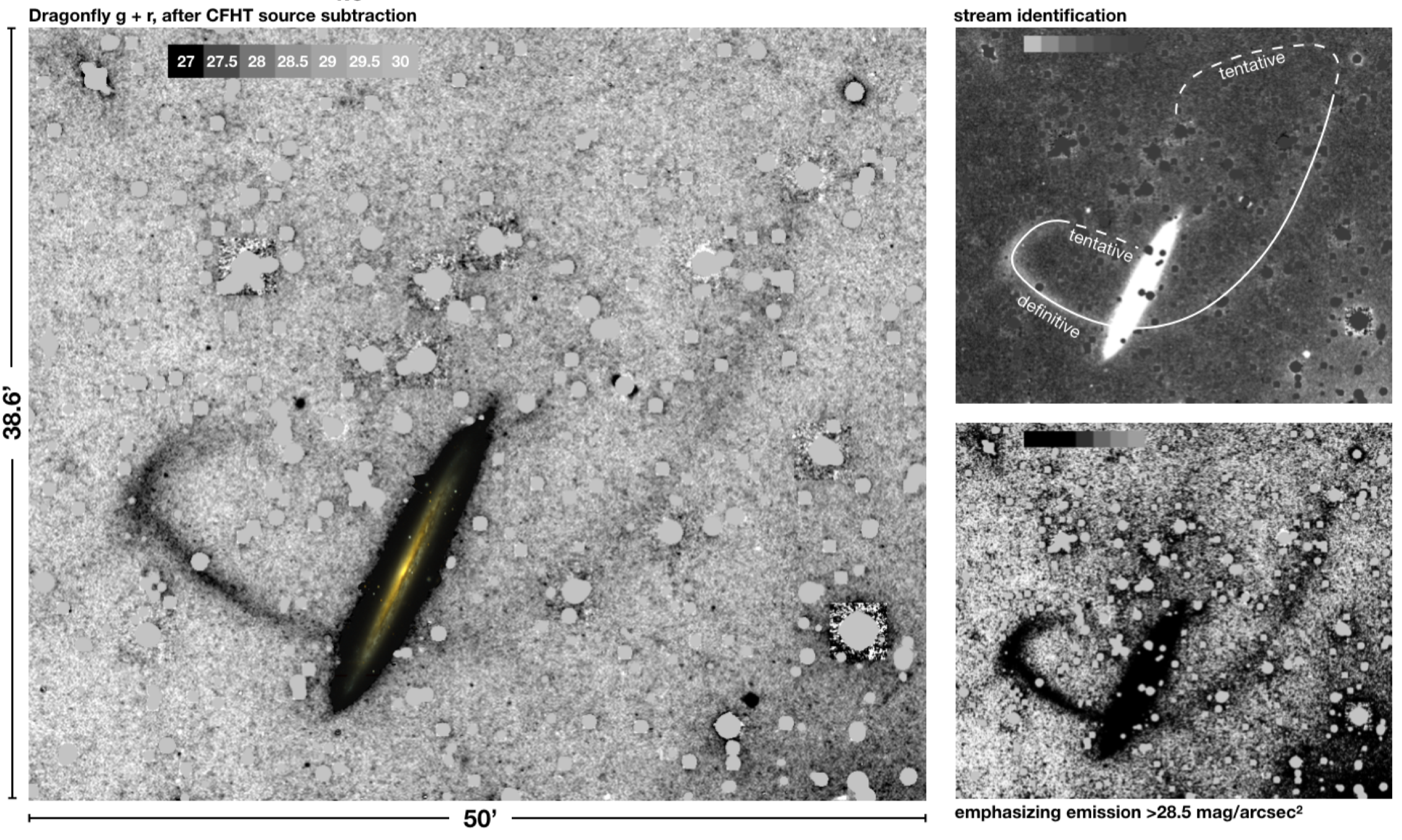
: NGC 5907 in the eye of Dragonfly

Pieter van Dokkum今天发了挺有意思的一篇小文章。NGC 5907是一个挺近 (17 Mpc) 的侧向 (edge-on) 星系，1998年一位中国天文学家用北京天文台的0.6/0.9m施密特望远镜发现了这个星系周围环绕着的一圈疑似潮汐瓦解遗迹的低面亮度特征🔗。而后这个星系又被很多人观测过，其中一位叫做Martínez- Delgado的业余天文学家在2008年也用他0.5m的RC望远镜拍了这个星系🔗 - 🔗，但是他们发现了两个“环”。十年过去了，Pieter van Dokkum领导的Dragonfly团队（就是发现缺少暗物质的星系的那个）又重新拍摄了这个星系，基本确认了NGC 5907在 29 mag/arcsec2 以上只有一个长长的右尾巴和一个90度拐角的左尾巴。而且Martínez- Delgado图中第一条”尾巴“的位置也跟Dragonfly和北京天文台拍的对不上。那么问题来了：到底是Dragonfly错了，还是那位业余天文学家错了呢？😏

这些痕迹的面亮度都非常暗（27-29 mag/arcsec2)，Dragonfly望远镜对“尾巴”细节的精确捕捉正体现出了Dragonfly对于探测低面亮度细节的强大威力。Dragonfly现在正在进行wide field巡天，而我也在写帮助他们更容易低面亮度特征的代码，期待以后会有更多有意思的发现。

(Link for emoji: emojipedia)

An introduction to astrophysical observables in gravitational wave detections

Introduction
- GW170817 (double NS) provides clues for the formation of elements heavies than iron (gold and platinum observed in the spectrum). It is also accompanied by a short GRB.
- GW only transfers very small amount of energy, hence it can penetrate very dense matter field.
Long story short
- The maximum observed NS is 2.1 solar mass. How did they form if single degenerate SN model is correct and Chandrasekhar is total right.
- NS is not totally made of neutron. It has lighter elements and iron (predominate) on the surface, and then heavier elements with more neutron, and then compact exotic matter (strange quark matter? @xrx) The EoS of NS has not been understood yet.
- A rotating BH comes from stellar collapse which has non-zero angular momentum before collapsing. There are many problems related to BH which remain mysteries now: mass function, mid-mass BH, etc.
Ground-based laser interferometers
- After the failure of Weber bar and knowing that strain from astronomical events is of magnitude of $h\sim 10^{-22}$, people began to build interferometers, including LIGO (USA, 4-km), Virgo (France and Italy, 3-km) and GEO (UK and Germany). More will be built in the near future (LISA, Tianqin, DECIGO, etc.)
- The interferometers are set up to make the interference destructive at the photodetector. Note that interferometer is only sensible to strain ($h\sim 1/r$), not to radiation power ($P\sim1/r^2$).
- LIGO is built to be sensitive in 20-20000 Hz, the noises are dominated by seismic on low-frequency end and quantum effects on high-frequency end.
- Optical system makes use of “Fabry-Perot cavities” to increase the distance light travels and “power recycling mirrors” to increase the power of laser light. LIGO uses 1064 nm infrared laser with ~40 W power. Mirrors are well designed, they only absorb one photon out of 300,000 photons, avoiding mirror heating, which could change the shapes of mirrors.
- The test masses are suspended by a passive damping system. LIGO also uses active (and kind of adaptive) damping system to fight against human-generated vibrations.
Double BH merger: GW150914
- GW150914 is the first GW event detected by human!! A brand new era of astrophysics started!
- LIGO people generate 250000 templates based on post-Newtonian and numerical relativity to fit the detected signals. Templates range from 1 solar mass to 90 solar masses. The S/N of GW150914 is 24.
- Based on Newtonian mechanics, during the inspiral process, we could estimate the chirp mass by $\omega$ and $\dot{\omega}$. And it turns out $\mathcal{M} \sim 30 M_\odot$. The coalescence stage begins when the Schwarzchild radius of two BHs contact with each other. For GW150914 the coalescence begins at $\nu\sim 330\ \text{Hz}$, so the total mass of two BHs can be estimated $M\sim 70 M_\odot$. Given chirp mass and total mass, the mass of two BH can be worked out: $m_1^{obs} = 42M_\odot,\ m_2^{obs} = 28 M_\odot$.
- The flux and total luminosity of binary BH merger can be given by GR. Hence we could derive the luminosity distance for this event $D_L = 400\ \text{Mpc}$. If we know the redshift (say from possible EM counterpart), we could yield a Hubble constant. Also, given this luminosity distance and LCDM cosmology, the redshift $z\sim 0.1$. Notice that cosmological effects (redshift and time dilution) affect the measurement of mass. In source coordinate, the mass is $m = m^{obs} / (1+z)$.
- GW150914 emits 4 solar mass energy within a tenth of second, however our sun emits 0.01 solar mass in 10 Gyr.
- After the ringdown process, a Kerr BH will be formed. Notice that a Kerr BH has smaller horizon area than a Schwarzchild BH of the same mass. Hence Kerr BH is more compact. The study of Kerr BH after ringdown could give us insights to strong field regime of gravity and further inspection of the validity of GR.
- The sky location resolution of LIGO is $\Delta \theta = \lambda / L \sim 28^{\circ}$ for this event.
GW170817, GRB170817A, AT 2017gfo
- Respectively - the GW event, the gamma-ray burst 1.7 s later, the afterglow in different wavelengths (kilonova).
- GW170817 - toward the end of the data run of O2 of aLIGO and aVirgo
- NS binary - produce a GW signal observable by ground-based detectors in the final minutes before the massive objects collide.
  - Detection rate for advanced detectors (per year) - $\mathcal{O}(0.1)\sim\mathcal{O}(100)$ (astrophysical uncertainty).
  - First indirect observation of GW - the Hulse and Taylor pulsar.
  - Position localization - 28 deg$^2$ (purely GW signal restriction).
  - Again, the chirp mass $\mathcal{M}$ ($\sim1.1\ M_\odot$ in the source frame and $\mathcal{M}^{d e t}=1.1977 M_{\odot}$ in the detectors frame when $z=0.008$ which) and the radius $R$ of the system are directly determined by observed $\omega$ and $\dot\omega$ during the inspiral phase. The amplitude $h$ is $\sim10^{-22}$ so we can derive a luminosity distance and redshift, which are consistent with the known results of NGC 4993
  - As $R$ approaches the size of the bodies, PN theory is no longer valid, relativistic effects related to the mass ratio $q=m_2/m_1$ (where $m_2>m_1$) as well as spin-orbit and spin-spin couplings become more significant. The derived chirp mass $\mathcal{M}$ differs from values at early times, which means the details of the objects’ internal structure become important.
  - Individual masses are more difficult to determined. By assuming high/low spins, the masses of both objects are approximately $1.4M_\odot$.
  - The inclination of the system $\theta \leq 28^{\circ}$.
  - Tidal effects are important for NS binaries (not important for BHs because they are bald as astronomers always do) especially when the two objects get really close, which corresponds to a high frequency $\nu_{g w} \simeq 600\ \mathrm{Hz}$. This is at present too hard for a ground-base interferometer to achieve, but once it is detected, we would gain a better understanding of the EoS of a NS.
  - The final state depends on individual masses. It can be a NS with a torus, a supra-massive/hypermassive NS which turns into a BH with a torus soon, or directly a BH with a torus.
- GRB170817A - the prompt emission is attributed to internal energy dissipation inside a relativistic jet (relativistic expanding fireballs)
  - Short GRB ($\Delta t \leq 2\ \mathrm{s}$) - first direct observation evidence.
  - 1.7 s later than the GW, which is consistent with models of NS mergers
  - The luminosity assuming an isotropic radiation is $\sim 4 \times 10^{46} \text { erg}$, which three orders of magnitude lower than a typical short GRB - a beamed emisson
- AT 2017gfo - afterglow of GRB170817A caused by forward shocks propagating in the surrounding ambient material and the related elemental decays
  - Atoms heavier than $\ce{Fe}$ are now able to form in r-process, where an atom captures neutrons rapidly enough to exceed the decay of neutrons. The complex absorption lines come from these new atoms.
  - The newly formed atoms then decay to emit thermal radiation, which leads to the afterglow.
  - By assuming all heavy atoms come from NS mergers and applying the heavy elements producing rate of AT 2017gfo ($\sim 0.05M_\odot$), we can estimate the event rate of (detectable) NS mergers, which is of $\mathcal{O}(1)\sim\mathcal{O}(10)$ within $\sim200$ Mpc. If too many similar events are detected, some refinements regarding the theoretical models would be necessary. If we are not able to detect such events that much, other mechanisms of heavy elements production may also be important.
Astrophysics of stellar BHs after GW150914

Until now we have detected a couple dozens of BH mergers. They are typically more massive that our past observed BHs (typically X-ray binaries). This challenges the formation theories of stellar mass BHs. We also observed a gap in the BH mass spectrum between 2.5 solar mass (below which are all neutron stars) and 5 solar mass. Also, we don’t find many intermediate-mass BHs.

Another very nice scientific outreach articles by Nature: How gravitational waves could solve some of the Universe’s deepest mysteries and How gravitational waves might help fundamental cosmology.

Yingjie: The Dependence of AGN Activity on Environment in SDSS

More massive galaxies are more likely to host AGNs than low mass ones. Some find that denser regions harbor AGNs more than low density regions, while some don’t think so. The use of different environment tracers may explain this dispute.

KIPAC: Statistical Methods in Astrophysics

05/20/19 - 05/26/19

Filippo Mannucci: The cosmic chemical evolution of galaxies

Metals are created by star formation and stellar explosions, dispersed by AGB and SNe and AGN feedback. Z increases with SF, decreases with metal-poor infalls and metal-rich outflows. Z could provide feedback and constrain SF timescale.

Different elements have different forming timescales.

Massive galaxy has higher alpha/Fe = short timescale.

How to measure Z?

Stellar metallicity (UV+opt+nearIR). Conroy uses spectrum fitting, but others may use indices (such as Dn4000 to indicate age). UV shows Z for OB stars, optical shows Z for redder stars. The difference can be such explained.
Hot ICM and CGM gas (X-ray)
Warm ISM (UV + opt + nearIR)

Mass-Metallicity relation: massive, high metallicity.

Why: less massive, shallower potential well. Massive galaxy, older, more accretion. IMF.

Peng 2015: about stellar Z.

Gas metallicity? Measure aurora lines in gas -> derive temperature -> derive metallicity??

MZR certainly goes down at high z.

MZR shows the efficiency of feedback of simulations.

Metallicity goes down with increasing SFR for given mass. This relation is invalid for high mass regime. This relation holds no matter for SDSS (single fibre for whole galaxy) or for IFU (valid in each spaxel). This relation is called fundamental metallicity relation FMR. What’s more, FMR doesn’t evolve with time. \

Ongoing projects: IFU metallicity, metallicity gradient.

Star formation quenching in massive galaxies

05/13/19 - 05/19/19

The Close AGN Reference Survey (CARS) Comparative analysis of the structural properties of star-forming and non-star-forming galaxy bars

05/06/19 - 05/12/19

B&R-4: South America is embracing Beijing’s science silk road

The investments on science is not clear and transparent enough. The Chinese way of doing things is top down, from government to organization to individuals. The western way is bottom up instead.
The concern of climate and environment is very necessary. It is said that the three-gorges dam in China has permanently changed the climate in west China, making more precipitation in the northwest China and severe and lasting drought in the southwest China. China has built a dam in Ecuador, but the environmental effect is unknown.

B&R-3: China charts a path into European science

It’s really clever that Chinese government will own infrastructures in poor nations in the future since they cannot pay back the loans. These infrastructures just provide standing points for the neo-colonialism of China. Thumbs up!

Deep+Wide Lensing Surveys will Provide Exquisite Measurements of the Dark Matter Halos of Dwarf Galaxies

04/29/19 - 05/05/19

B&R-2: Scientists in Pakistan and Sri Lanka bet their futures on China

China is developing close scientific cooperation with Pakistan and Sri Lanka, on food security, railway, infrastructure construction, epidemiology, medicine, etc.

B&R-1: How China is redrawing the map of world science

字里行间充满了酸溜溜的味道。
环境问题确实很重要，值得引起重视。

Nature: The new physics needed to probe the origins of life

Low-mass black holes as the remnants of primordial black hole formation

Astro2020 Science White Paper: The Local Relics of of Supermassive Black Hole Seeds

We have detected supermassive BHs and stellar-mass BHs. We found a SMBH with $M>10^9 M_\odot$ at $z>7$. But we know nothing about how they form. The intermediate-mass BHs ($100 - 10^5\ M_\odot$) could serve as seeds for the formation of SMBH. We didn’t find any IMBH so far.
One speculation is that IMBH is in the center of GC. Taking the advantage of high resolution of next generation ground-based large telescopes (TMT, E-ELT), we could measure the proper motion of stars in the center of GCs at different epochs, then derive the mass of central BH. The existence of $10^3\ M_\odot$ BH could increase the central velocity dispersion by 1 km/s.
Another possibility is that IMBH is in the center of low-mass galaxies. Using IFU + adaptive optics on 8-10 meter telescopes, we have already made progress on the demography of SMBH. In the same way, we could measure the $\sigma^*$ with much higher resolution for nearly all low-mass galaxies.

04/22/19 - 04/28/19

Drawing an elephant with four complex parameters

With four parameters I can fit an elephant, and with five I can make him wiggle his trunk. — von Neumann

Surface Brightness Fluctuations

References: Lecture slides of Rolf Kudritzki; Chapter 4.2 of Richard de Grijs book.

We always (typically) use ETG to measure surface brightness fluctuations. (Any chance that we can use UDG or disks? I remembered that one of Jenny Greene’s students wrote a paper about this.) We could resolve individual stars in M32, so the Surface Brightness (SB) is fluctuating across the image. It’s easy to understand that it would be very smooth if we put that galaxy to very far away.

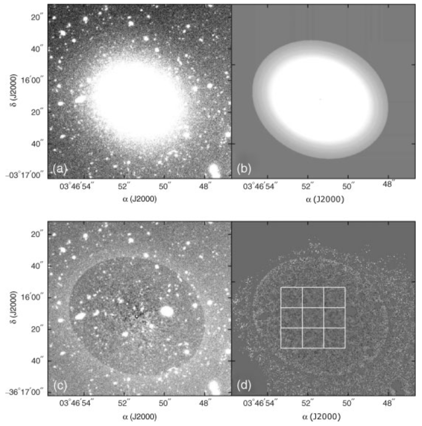
: Image reduction for SBF measurement. (Fig 4.2, de Grijs book)

Given the luminosity function, we could divide stars in galaxy into several separated parts, hence $L = \sum n_iL_i$. Now we only focus on one part of them. Assuming the pixel scale is $\theta$ on the sky, the distance is $d$, the column density of stars is $n_i$, thus the number of stars you see in each pixel is $N_i = n_i (d \theta )^2$. The flux we received from these stars is

\[F_i = \frac{N_i L_i}{4\pi d^2} = \frac{n_i L_i \theta^2}{4\pi}=\mathrm{const.}\]

That is to say that surface brightness (often expressed in mag/arcsec^2) remains a constant, regardless of distance.

Assuming the Poissonian fluctuations of number of stars, we have: $\sigma_{F_i}/F_i = 1/\sqrt{N_i}$, thus

$\frac{\sigma_{F_i}^2}{F_i} = \frac{F_i}{N_i} = \frac{L_i}{4\pi d^2} \propto \frac{1}{d^2}$.

We define the surface brightness fluctuation to be $\sigma_{F_i}^2/F_i$, it goes as $d^{-2}$.

If we consider all stellar populations: (note that $\sigma_{F_i} = \left(\frac{\theta}{4\pi d}\right)^2 n_i L_i^2$ )

: Power spectrum of the image and SBF

$\sigma_F^2 = \sum \sigma_{F_i}^2 = \left(\frac{\theta}{4\pi d}\right)^2 \sum n_i L_i^2$,

$F = \sum F_i = \frac{\theta^2}{4\pi} \sum n_i L_i$.

Thus $F_{SBF} = \frac{\sigma_F^2}{F} = \frac{1}{4\pi d^2}\frac{\sum n_i L_i^2}{\sum n_i L_i}$. As long we get $F_{SBF}$ for two galaxies with almost the same stellar population, we could derive the distances ratio of these two galaxies using SBF method. However, the calibration is not trivial.

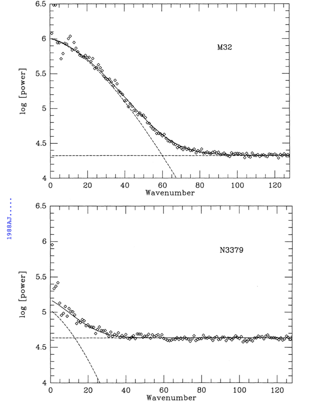
How to measure the SBF? For an elliptical galaxy, first you need to fit a overall (2-D) model for the smoothed light distribution. After subtracting this model from image, the fluctuation is left. You can also normalize the fluctuation and mask out contaminations (see lower-right panel). Then you need to apply Fourier transformation to the image and derive a power spectrum. It will look like:

\[|I(k)|^2 = \sigma_{SBF}^2 P_{\mathrm{PSF}}^2(k) + \mathrm{const.}\]

The PSF term is easy to understand, since the pixels within the FWHM of PSF is kind of correlated. The constant term comes from the random fluctuations from sky, ccd bad pixels, cosmic rays, etc. (since the modulus of Fourier transform of a delta function if a constant). In the following figure, upper panel is M32 at 8 Mpc, where lower panel is NGC 3379 at 10 Mpc. The declining dashed line shows the power spectrum of PSF. Comparing both panels, the effect of $\sigma_{SBF}^2$ is significant, making it the good tool to indicate distance for nearby elliptical galaxies.

04/15/19 - 04/21/19

CSST Workshop

The following is from the presentation of Luis Ho.

CSS will be launched in 2022, three astronauts living in orbit. Tiangong station has 39 boxes, only one of those boxes is used in applied sciences. CSST will be launched in 2024.

If you mount the telescope onto to space station, the vibration will decrease the image quality. Brilliant idea: fly the telescope in the same orbit, so that the telescope could be mounted into the CSS anytime, making changing instruments and repairs possible and feasible.

Europe will launch Euclid (2.4m, PSF = 2 arcsec), aiming at cosmology and weak lensing. US is also considering launch WFIRST (near IR), the future of it is not clear.

On the ground, we will have LSST (8m), survey in time domain. LSST and CSST is complimentary, CSST will have higher resolution.

Optical design: 离轴三反 (clear PSF, good for weak lensing). It has almost the same number of pixels as LSST camera (largest one ever built).

CSST Imaging: 17500 Wide mode, 255-1000nm, more than 6 filters (SED coverage, from near UV to J band), 0.15 arcsec seeing. CSST Spectroscopy: R>200 (better than typical narrow band). “Huge area, large wavelength coverage”

Sciences: Cosmology (lensing, very good photo-zs, large scale structures), AGN/Galaxies, etc.

CSST is $7500\times 7$ COSMOS (since COSMOS is only 1 square degree and is only in $i$ band.

Problems: We don’t have a good team. (Euclid and WFIRST have big teams, complete docs).

“To the zero/first/second order, CSST = HST”. To do science, we don’t need 17500 deg^2. “LSST = HSC”.

“CSST + Euclid + WFIRST = CANDELS (many bands, near complete SED data)”

We can think about combining HSC data and their overlap with previous data.

“What do you measure and how do you measure???” (Tidal tails, UDGs, meters, etc.)

Best way to prepare for CSST: the only driven source is to write papers and pipelines.

Planning the scientific applications of the Five-hundred-meter Aperture Spherical radio Telescope

FAST has already done the first commission called CRAFTS (Commensal Radio Astronomy FAST Survey). CRAFTS observes pulsar, HI galaxy, HI image, fast radio burst (FRB) and other transients in radio band.
FAST could measure the fundamental constants of nature, and explore the physics behind cosmic rays, gravitational radiation, pulsar magnetospheres, interstellar masers, etc.

04/08/19 - 04/14/19

The supernova rate per unit mass

Ensemble photometric redshifts

The Universal Stellar Mass-Stellar Metallicity Relation for Dwarf Galaxies

Coordinated Assembly of Brightest Cluster Galaxies

Related to my ICL project.

$[\alpha/\rm{Fe}]$ is used to indicate the star formation (burst) timescales. We know that after the starburst, SNe II explode promptly and produce a large amount of $\alpha$-elements (such as O, Ne, Mg, Si) and relatively less iron. Several time (1 Gyr) after the starburst, SNe Ia start to explode and produce a large mount of iron.

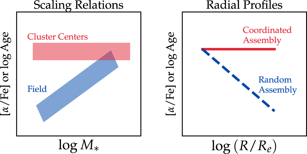
: Coordinated Assembly of BCG (Gu et al. 2018a)

Observations show that massive galaxies (region) are older, more metal-rich, more $\alpha$-enhanced compared to low-mass galaxies. They also have higher velocity dispersion in the center. We know that low-mass galaxies are possibly the building blocks of very massive galaxies. However, these building blocks have low metallicity and low $\alpha$ abundance, thus they would dilute the metallicity and $\alpha$ abundance of massive galaxies, making it a paradox. However, the relations between $M_*$ and metallicity ($\alpha$ abundance) have large scatter. There are some low-mass galaxies which are old, metal-rich and $\alpha$-enhanced. Hence it seems that massive galaxies are prone to gather their building blocks which have early truncated star formation and have high $\alpha$ abundance. This assembly is called Coordinated Assembly of BCG by this paper.
This paper utilizes MUSE IFU data to explore chemical abundances and velocity dispersions in galaxy cluster Abell 3827. In this cluster, there are several galaxies which will merge together within 1 Gyr. For these galaxies, their centers are old, have high $[\rm{Fe/H}]$ and anomalous high $[\rm{\alpha/Fe}]$. So this paper proposes that the building blocks are environmentally quenched. The star formation (burst) before was short, and early???

Spectroscopic Constraints on the Build-up of the Intracluster Light in the Coma Cluster

Related to my ICL project.

Tools for studying ICL: multi-band photometry; spectroscopy; IFU; globular clusters; planetary nebulae or other individual objects; red giants branch stars.
alf (developed by Charlie Conroy and Pieter van Dokkum) is able to fit a two burst star formation history, the redshift, velocity dispersion, overall metallicity [Z/H], 18 individual element abundances, several IMF parameters, and a variety of nuisance parameters. This paper uses top-hat priors for most of parameters.
For a typical ETG, the velocity dispersion in the central region is 200-300 km/s, and the velocity dispersion in the ICL region is above 400 km/s.

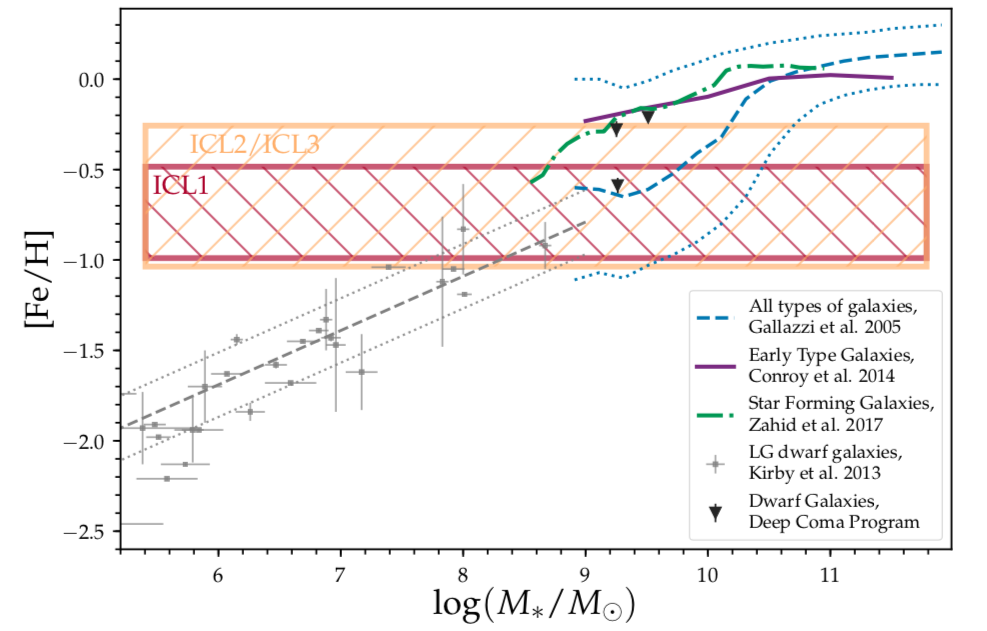
: Stellar Mass - Metallicity Relation (Gu et al. 2018b)

“Both BCG + ICL $g-r$ colors become bluer with increasing radius. This is consistent with our spectroscopic results that the stellar population is more metal poor with increasing radius.”
The SNR could be expressed like SNR density: in the unit of $\mathrm{nm}^{-1}$.
“Both BCGs+ICL structures have rising velocity dispersion profiles, suggesting that stars in the ICL trace the potential of the Coma cluster instead of any individual galaxy. “ “Nearly flat stellar age profiles in ETGs are observed.” “The massive ETGs in the central regions of galaxy clusters grow by accreting preferentially old stellar systems”
Possible mechanism of ICL: tidal disruption of dwarf galaxies; tidal striping of low mass galaxies through galaxy interactions; violent relaxiation during major mergers; in-situ star formation.
On the assembly of ICL. Basically two stage formation of BCG: in-situ star formation in high-z; accretions and mergers in low-z. We already have an established relation between stellar mass and overall metallicity (MZR). More massive galaxy has higher metallicity. The metallicity of ICL here measured by MaNGA indicates that: if they comes from individual galaxies, they should come from dwarf galaxies with stellar mass $8 < \log(M_*/M_\odot) < 9.5$. Noticing that the metallicities of BCG outskirts are relatively low, hence another possibility is that the ICL stars come from outskirts of BCG. But they are unlikely come from the inner part of massive (both disk and ETG) galaxies (say $\log(M_*/M_\odot) > 11$).

dynesty: A Dynamic Nested Sampling Package for Estimating Bayesian Posteriors and Evidences

EDGE I: the mass-metallicity relation as a critical test of galaxy formation physics

Cook: Measuring Star-Formation Histories, Distances, and Metallicities with Pixel Color-Magnitude Diagrams I: Model Definition and Mock Tests

04/01/19 - 04/07/19

Fast interstellar dust extinction laws in Python

Intracluster light: a luminous tracer for dark matter in clusters of galaxies

Effects of Gas on Formation and Evolution of Stellar Bars and Nuclear Rings in Disk Galaxies

Interesting one. TO READ.
We still do not know/not sure wheter the formation (time) of bar is correlated to the gas content $f_{\rm gas}$.

TESS Photometric Mapping of a Terrestrial Planet in the Habitable Zone: Detection of Clouds, Oceans, and Continents

They use starry package to fit albedo map on the exoplanet and find continents on it! Check the image here!

ACRONYM: Acronym CReatiON for You and Me

pip install acronym and get fantastic acronyms for your projects!

Filter Profile Service: A repository of Filter information for the VO

03/24/19 - 03/31/19

天文物理类英文科技论文写作的常见问题

Super useful!!!!!

The Information Content of Stellar Halos: Stellar Population Gradients and Accretion Histories in Early-type Illustris Galaxies

Kormendy: Secular Evolution in Disk Galaxies

Belfiore 2018: SDSS IV MaNGA – sSFR profiles and the slow quenching of discs in green valley galaxies

Andy Goulding: Galaxy-scale Bars in Late-type Sloan Digital Sky Survey Galaxies Do Not Influence the Average Accretion Rates of Supermassive Black Holes

Spinoso 2019: Bar-driven evolution and quenching of spiral galaxies in cosmological simulations

SDSS-IV MaNGA: Spatially Resolved Star Formation Main Sequence and LI(N)ER Sequence

03/17/19 - 03/23/19

Illuminating Low Surface Brightness Galaxies with the Hyper Suprime-Cam Survey

Blends of faint galaxies and/or distant galaxy groups are a major source of contamination for any deep diffuse-galaxy search (e.g., Koda et al. 2015; Sifón et al. 2018). The faintness of these sources means that they will not be masked by the previous step of our pipeline, and if detected as single objects, their sizes will be biased high and their central surface brightnesses will be biased low, making them look like the objects we are searching for.

Belfiore 2016: SDSS IV MaNGA – spatially resolved diagnostic diagrams: a proof that many galaxies are LIERs

IMPORTANT for my paper!

People used BPT diagram to distinguish SF galaxies with AGN galaxies. But in the past, SDSS only uses single-fibre spectrum, whose aperture typically corresponds to several kpc (also considering seeing). But to confirm AGN, you need to zoom more in to the scale of ~ 100 kpc.
“Heckman (1980) first presented a detailed study of LI(N)ER emission, arguing that LI(N)ERs could represent the low-luminosity extension of the Sy population. Studies of the central few parsecs in nearby galaxies (Ho, Filippenko & Sargent 1997; Shields et al. 2007) demonstrate that LINER emission on those scales can be associated with nuclear accretion phenomena, in particular weak, radiatively inefficient AGNs (see for example the review from Ho 2008). “ But Belfiore argued that the H$\alpha$ emission luminosity excited by pAGB stars can be equal to (or brighter than) that excited by LLAGN. So pAGB can be a strong candidate.
The demarcation line between SF and Seyfert+LINER can be derived theoretically. Here we use Kauffmann 2003 and Kewley 2001 (dotted in my plot). “The [S II] BPT diagram is not affected by the N/O abun- dance ratio, and provides a cleaner separation within the ‘right-hand sequence’ between Sy and LIERs (Kewley et al. 2006)”. The demarcation line between Seyfert and LINER is from Kewley 2006.
Stars in LINER region are typically older than other regions. Stars in LINER region with larger S[II]/H$\alpha$ are older.
cLIER: central (within one PSF at least) LIER (classified by S[II] BPT); eLIER: LIER extends to one PSF at least; Seyfert: AGN within PSF; Line-less: EW[H$\alpha$] < 1 within $1 R_e$.
More cLIER and more eLIER at high mass end, more SF at low mass end.
They study H$\alpha$ profile and EW profile. SF has high EW, eLIER has low EW, cLIER has low EW at center, and EW increases rapidly.
cLIER and eLIER are supported by pAGB star because: 1. Old stellar population; 2. low EW and flat gradient. The gradients of ionization parameters also rules out AGN as sources of eLIER.

Voronoi bin: Adaptive spatial binning of integral-field spectroscopic data using Voronoi tessellations

Implement Voronoi bin in Python: VorBin.
Michele Cappellari has written so many packages!!!

HI galaxies with little star formation: an abundance of LIERs

They selected 91 HI galaxies with no (or little) star formation from a HI survey. They study the IFU data of some of them, classify them into SF, Seyfert, LINER and LIER. They find most (75%) of these galaxies are LIER.
D4000 data implies that LIER region has an average stellar population age ~ 5 Gyrs. Given that pAGB stars come to power 2 Gyrs after the last star formation event (Belfiore 2017), this paper supports the post AGB scenario.

03/11/19 - 03/17/19

Subo Dong’s talk on Supernovae

Kinetic energy is $10^{51}$ erg.

Radiation energy is $10^{49}$ erg.

10000 km/s is the typical velocity for SN explosion.

Zwicky: pioneer of searching SN.

SN1987A: in LMC, but is type II.

Gravitational binding energy: $10^{53}$ erg. Where has energy gone? Neutrino!

Neutrino energy: $10^{53}$ erg.

We still don’t know the explosion mechanism of CC SN

Detection power: $A(\mathrm{m}^2)\times\Omega(\mathrm{deg}^2)$, and LSST stands out!

SNe Ia are the “main sequence” of SNe, they are regularity and continuous.

Type II and Type Ib/Ic trace star formation. Type Ia doesn’t depend on environment too much.

The light of SN comes from $^{56}\mathrm{Ni}$ decay. Low luminosity Ia are from elliptical galaxies, on the contrast, Ia in spirals are more luminous. Every theory should be able to produce an order of magnitude difference of Nicole. 1991bg: low luminosity; 1991T: super luminosity.

We don’t know how to trigger the explosion. (Maoz et al., 2014 ARAA); Duran Kushnir, Boaz Katz, Dan Maoz

Try to find close WD pairs as SN progenitors: SPY survey.

Subo: major channel WD-WD direct collision. ~ 20% WD in triples can explain the major channel of SN Ia.

Long time to produce low mass WD, thus more sub luminous Ia in ETG.

Just explode: we only see photosphere, ejecta are optical thick. With time goes on, we see deeper into that. After months, the ejecta gets nearly transparent, and turns into nebular phase.

Smoking gun paper: using cobalt line and found bimodal velocity distribution. Two chunks of Ni56! Fraction: 3/20. But viewing angle should be taking into consideration!

Non-equal mass of WD pairs leads to blueshift-redshift of cobalt lines.

Ping’s new work: H$\alpha$ line, thin, less than 200 km/s. Maybe Ia-CSM?

03/04/19 - 03/11/19

The distance, supernova rate and supernova progenitors of NGC 6946

We can estimate the SFR over the last $\sim 100$ Myrs using core-collapse SNe rate. This is only the lower limit of SFR since there are more missed or failed CC-SNe that we didn’t see.
Given a SFR and metallicity, one can calculate the FUV luminosity of a galaxy. After applying extinction (both from the foreground and intrinsic) corrections and comparing it with observation, a luminosity distance can be determined.
The distance to SN is crucial for determining the intrinsic luminosity of it. Larger distance here implies brighter/more massive progenitors. Using the new distance, two events become normal and can be explained from stellar physics models. Distances should be paid attention to!
The homepage of first author: Dr. J. J. Eldridge

On Stellar Population Synthesis:

Modeling the Panchromatic Spectral Energy Distributions of Galaxies

How to measure galaxy star-formation histories I: Parametric models

How to measure galaxy star formation histories II: Nonparametric models

Stellar population synthesis at the resolution of 2003 (BC03)

02/25/19 - 03/03/19

The NANOGrav 11-Year Data Set: Limits on Gravitational Waves from Individual Supermassive Black Hole Binaries

Just read this astrobite on this paper.
NANOGrav project provides another approach of detecting gravitational waves. LIGO (and other ground-based experiments) is sensitive to high-frequency GW (1-1000 Hz), which is usually excited by binary BH mergers or binary NS mergers. Pulsar timing array is sensitive to low-frequency GW (nano-Hz), usually excited by the merger of supermassive BHs which are the result of galaxy-galaxy mergers.
(Submilimeter) Pulsar is the lighthouse in the universe. If the gravitational wave propagate in the direction from the pulsar to us, the period of pulsar will be slightly different. This paper analyzes the past 11-year data from 43 pulsars, and find no GW event above a certain strain.

We find that there are no SMBHBs with a chirp mass greater than $10^9$ solar masses within a distance of 120 Mpc and none with chirp passes greater than $10^{10}$ solar masses within 5.5 Gpc. Using this data set, the collaboration has determined that there are no SMBHBs in the Virgo Cluster with a chirp mass greater than $1.6 \times 10^9$ solar masses emitting gravitational waves at a frequency of 9 nHz, which implies that none of the galaxies NGC 4472, NGC 4486, or NGC 4649 (which are all candidates for gravitational waves in the Virgo Cluster) could contain SMBHBs emitting gravitational waves in this frequency range.
I know very little about this area. But it will be quite exciting if we detected the GW from SMBHs merger in the nearby galaxies.

A Brief History of Gravitational Waves

The discovery of the first GW event is quite interesting and exciting. It’s worth noting that ‘inject’ events test the correct judgment of GW events.
Unlike electromagnetic wave, which can be excited by electric dipole (one positive, one negative), the gravitational wave cannot be simply excited by a dipole, since there’s nothing with negative mass.
Imagine we have two points A and B. We can only detect the transverse GW which is propagating perpendicular to A-B. Only this type of GW could stretch the distance between A and B. The best ‘ruler’ of measuring distance is light. The speed of light is constant and unaltered by a gravitational wave.
Richard Feynmann designed a gedanken experiment to show that gravitational waves do carry energy. “I was surprised to find that a whole day of the conference was spent on this issue and that ‘experts’ were confused. That’s what happens when one is considering energy conservation tensors, etc. instead of questioning, can waves do work?”
Joseph Weber designed the very first GW detector, names “Weber bar”. But limited by the suspension techniques and thermal noise isolation, Weber published wrong results of detections. This kind of intense GW comes from the central SMBH of milky way will make our galaxy disperse before we human beings exist.

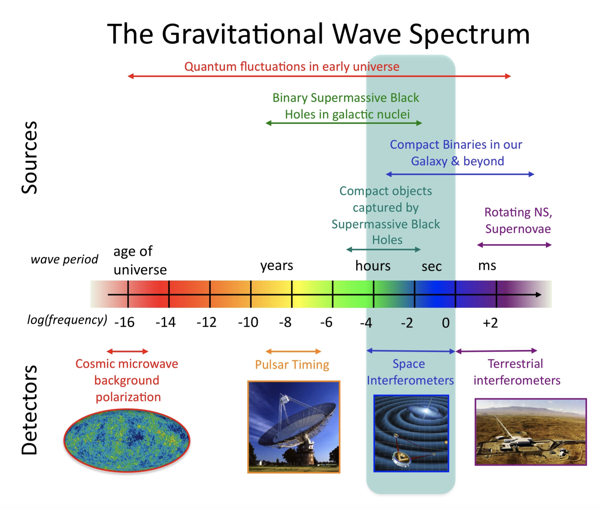
: Gravitational wave spectrum showing wavelength and frequency along with some anticipated sources and the kind of detectors one might use. Credit: NASA Goddard Space Flight Center.

The coalescences between stellar mass black holes produces GW with the amplitude of $h = 10^{-21}$.
In designing an interferometer to detect GW, the optimal size of the arms is one-forth of the GW wavelength. (100 Hz corresponds to 750 km) Rainer Weiss came up with the idea of building an interferometer to detect GW in an undergraduate seminar on GR in MIT.
Prior to LIGO, German has constructed a 600-m interferometer called GEO-600 (1994), which contributed a lot to this industry. France and Italy also built VIRGO (2003) detector at the same time with LIGO.
Weiss cooperated with Thorne and Drever (both from Caltech) on building LIGO at first, but difficulties emerged between Weiss and Drever. Latter Barish took the position of Drever and became the leader of LIGO. He founded the laboratory LIGo and scientific collaboration LIGO, separately.
“Initial” LIGO runs from 2002 to 2010 but got no results. But right before the official run of “Advanced” LIGO, a GW from BH-BH merger was detected by aLIGO during an experimental run. After then, more and more GWs are detected by LIGO. Weiss, Thorne and Barish were awarded 2017 Nobel Prize in Physics. The new era has come.

02/18/19 - 02/24-19

The local and distant Universe: stellar ages and $H_0$

Hubble tension again. We measure $H_0$ from different aspects, but mainly from local distance ladder and CMB. The measurement of $H_0$ by using CMB is heavily based on $\Lambda$CDM model and basic physics in the early Universe. In the middle between CMB and local universe, SNe and BAO take part in. (Also notice that CMB could be used to probe all the physics from last scattering surface to today.) The determination of $H_0$ on local universe is based on some stellar physics (Cepheids, supernovae Ia). Note that local distance measurement relies on the flatness of Euclidean space. Gravitational Wave and counterparts, time-delay lensing,

To be read.

Dependence of Type Ia supernova luminosities on their local environment

I just read this astrobite about this paper.
People used to calibrate SNe Ia using color (B-V) and $m_{15}$. Now this paper suggest that the color of local environment of SNe (their surroundings) should also be considered as a factor of calibration. Redder color implies low SFR. Previous analyses have found that galaxies that are not forming many stars tend to host SNe Ia that are brighter than SNe Ia from very active galaxies even after standardization.
They test the distribution of Hubble residual $\mu - \mu_{model}$ for SNe in different local environments (different $U-V$ color). They find significant difference ($7\sigma$).
Hence, while calibrating things, we should not only consider the things themselves, but also the environments where they’re located.

WFIRST, The Wide Field Infrared Survey Telescope: 100 Hubbles for the 2020s

Scientific goal: weak lensing survey; find exoplanets by transient/microlensing and direct imaging (using coronagraph); supernova Ia survey and monitoring; general observation by submitting proposal. No data protection!
Really Wide Field! WFIRST can do COSMOS survey x125 faster; CANDELS-Wide 1050x faster; 3D-HST 730x faster. (See Fig. 2 in this paper)
Nice video about WFIRST: WFIRST: The best of both worlds.
WFIRST can discover (we hope so) 20,000 galaxies with $z>8$ (at the age of 0.6 Gyr) per month, 100 exoplanets per month, and about 8000 SNe Ia in total.

01/21/19 - 01/27/19

A second galaxy missing dark matter in the NGC1052 group, by Pieter van Dokkum group

01/14/19 - 01/20/19

SDSS-IV MaNGA: Inside-out vs. outside-in quenching in different local environments

The MASSIVE Survey - XII Connecting Stellar Populations of Early-Type Galaxies to Kinematics and Environment, by Jenny Greene

A mass-dependent slope of the galaxy size-mass relation out to z~3: further evidence for a direct relation between median galaxy size and median halo mass, by Pieter van Dokkum group

Continued from the following paper, which says $r_{80}$ may be related to galaxy halo. This paper studies this further and gets some interesting results. After reading this paper, I feel intensively that good science is linking difference fields. Dirac linked analytical mechanics (Poisson brackets) with quantum phenomena, then quantum mechanics was born. This paper superficially links the stellar mass - $r_{80}$ size diagram with the well-known stellar mass - halo mass relation, and get some interesting (maybe wrong, maybe correct) results.

Miller et al. 2019 already shows that the stellar mass - $r_{80}$ size diagram cannot tell the SF and passive galaxies apart. Fig. 1 shows that the median lines of stellar mass - $r_{80}$ size diagram are like two pieces of power law. Then they fit this ‘broken power law’ and define the pivot mass $M_{p}$, where the line turns up a little bit.
Then they find the pivot mass evolve with redshift significantly. The first slope (which is lower) changes slightly over redshift, but the second slope changes much. Actually the first slope (piece) is just composed of the passive galaxy branch, and the second slope (piece) is presented by SF galaxies.
Most interestingly, they remind of the stellar mass - halo mass relation. If the x-axis is stellar mass and y-axis is halo mass, the SMHM relation resembles this stellar mass - size diagram in $r_{80}$. So what’s the physics behind this? First, the halo mass is proportional to the cubed virial radius $R_{vir}$. And if $r_{80}$ is proportional to $R_{vir}$, then it’s reasonable that $r_{80}$ is a proxy of halo mass. So they just fit this coefficient for the most nearby redshift bin and find $r_{80} = 0.047 R_{vir}$. Assuming this holds for all redshift ranges, they plot SMHM relation predicted by $r_{80}$, which is now a proxy of halo mass. They find it’s good to $z\sim 2$.
In measuring the SMHM relation, there are many methods such as g-g lensing and clustering (which is more direct and more observational), abundance matching, and halo occupation distribution. But different methods gives different results and have different detection ability on redshift. They author also define a pivot masses for the SMHM relations and study their evolution. They don’t match with stellar mass - size one. So they suspect the intrinsic scatter may cause huge caveat when convert a halo-to-stellar relation to stellar-to-halo relation.

A New View of the Size-Mass Distribution of Galaxies: Using $r_{20}$and $r_{80}$ instead of $r_{50}$, by Pieter van Dokkum group

The classfication of galaxies can not only based on stellar mass - color diagram (also stellar mass - SFR diagram), bust also based on stellar mass - size diagram. In the past, people usually use the effective radius $r_{50}$ as a proxy of galaxy size. (But I have been suspecting how well can $r_{50}$ describe the size of a galaxy for a long time.) As a common sense, massive elliptical galaxies are more extended in the outskirts, but spirals are not. If we fit a galaxy using a single Sersic model, ellipticals tend to have larger Sersic index $n$. In this paper, Pieter and his collaborators check what would happen if we use $r_{20}$ and $r_{80}$ as proxies of galaxy sizes. And I remember that Sandy Faber talked about this quite a lot in a colloquium in KIAA.

This paper is quite straightforward. (But I didn’t dig deep into the sample selection part.) They find that if we use $r_{20}$, then using the stellar mass - size diagram can easily distinguish star-forming and passive galaxies apart. But using $r_{80}$, SF and passive behaves similarly.
In this paper, authors use some new algorithms/terms in statistics: Hartigan’s dip test; Gaussian mixture models; Bayesian information criterion; Ashman’s $D$ parameter; Kolmogorov-Smirnov test. But actually these are also straightforward.
They suspect $r_{20}$ has something to do with star-forming / quenching. Since $r_{80}$ is not very different between SF and passive galaxies, it may be related to the galaxy halo.
Besides, I find that log-normal distribution is interesting, see this paper Log-normal distributions across the science: keys and clues.

Still Missing Dark Matter: KCWI High-Resolution Stellar Kinematics of NGC1052-DF2, by Pieter van Dokkum group

On how to measure the velocity dispersion directly from spectrum, I found a paper by Luis Ho in 2002: A Study of the Direct Fitting Method for Measurement of Galaxy Velocity Dispersions. The main idea in this paper is:

In measuring velocity dispersion, it’s convenient to use $x = \ln(\lambda)$ scale, because $x' = \ln[\lambda(1+z)] = x + \ln(1+z) \approx x + z$ for $z\ll 1$.
Find some spectrums of stars as templates. They don’t have any velocity dispersions (or can be ignored).
Assume the effect of velocity dispersion is Gaussian. Then, to get a dispersed spectrum, you should convolve the template with a Gaussian kernel with a given radius. Write this in maths, that is $T(x)]\otimes G(x, r)$.
But we should consider that the featureless continuum components are different between template and galaxy. So we simply add a featureless continuum which is typically a straight line with $x = \ln(\lambda)$ (in $\lambda$ domain this is an exponential continuum). Hence: $[T(x)\otimes G(x, r)] + C(x)$.
To compensate other effects such as reddening difference between template and galaxy, we multiply a low-order Legendre polynomial, then get the final model spectrum. That is: $M(x) = \{[T(x)\otimes G(x, r)] + C(x)\}\sum_l P_l(x).$
Then we have several parameters, like Gaussian kernel radius, continuum straight line intercept and slope, and coefficients for every order Legendre polynomials. Note that in $\chi^2$, the error term contains the measurement error of galaxy spectrum, and error of template which is typically negligible. At last, let MCMC be. The radius of Gaussian kernel should be the velocity dispersion (need a conversion).

Now for the NGC1052-DF2 case, Shany make a spectrum combining spectrums of all special region. And this spectrum has been broadened. Shany uses templates from two Global Clusters, say M3 and M13. The templates here has already been broadened by velocity dispersion (Gaussian). And we know the $\sigma$ of two Gaussian obeys $\sigma_{\mathrm{star}}^2 = \sigma_{\mathrm{template}}^2 + \sigma_{\mathrm{measure}}^2$, where $\sigma_{\mathrm{star}}$ is the velocity dispersion of DF2. So we can measure $\sigma_{\mathrm{measure}}$ by the same method as stated above, and then get the velocity dispersion of DF2 $\sigma_{\mathrm{star}}$, which is $\sigma_{\mathrm{star}} = 8.4\pm2.1\ \mathrm{km s}^{-1}$.

How to calculate the dynamical mass given the velocity dispersion? I need to figure out.

Intrinsic shape or rotation axis (minor axis rotation.)

Kevin: it’s not necessarily weird that we detect a galaxy lacking dark matter in its central region. Given the large scatter of halo mass and halo concentration of a given stellar mass in the low-mass end, it’s probably that we just encountered a galaxy with low halo mass and low halo concentration.

Gaussian process

http://www.gaussianprocess.org/gpml/chapters/RW.pdf

Vox Charta Key: jiaxuan_li@PKU

Convert LaTeX to html gif picture: https://www.codecogs.com/latex/eqneditor.php