Notes on Review papers

Feel very ashamed for the decadence in the past year 2018. I will try to read as many paper as possible and do my best in 2019.

An introduction to astrophysical observables in gravitational wave detections

Introduction
- GW170817 (double NS) provides clues for the formation of elements heavies than iron (gold and platinum observed in the spectrum). It is also accompanied by a short GRB.
- GW only transfers very small amount of energy, hence it can penetrate very dense matter field.
Long story short
- The maximum observed NS is 2.1 solar mass. How did they form if single degenerate SN model is correct and Chandrasekhar is total right.
- NS is not totally made of neutron. It has lighter elements and iron (predominate) on the surface, and then heavier elements with more neutron, and then compact exotic matter (strange quark matter? @xrx) The EoS of NS has not been understood yet.
- A rotating BH comes from stellar collapse which has non-zero angular momentum before collapsing. There are many problems related to BH which remain mysteries now: mass function, mid-mass BH, etc.
Ground-based laser interferometers
- After the failure of Weber bar and knowing that strain from astronomical events is of magnitude of \(h\sim 10^{-22}\), people began to build interferometers, including LIGO (USA, 4-km), Virgo (France and Italy, 3-km) and GEO (UK and Germany). More will be built in the near future (LISA, Tianqin, DECIGO, etc.)
- The interferometers are set up to make the interference destructive at the photodetector. Note that interferometer is only sensible to strain (\(h\sim 1/r\)), not to radiation power (\(P\sim1/r^2\)).
- LIGO is built to be sensitive in 20-20000 Hz, the noises are dominated by seismic on low-frequency end and quantum effects on high-frequency end.
- Optical system makes use of “Fabry-Perot cavities” to increase the distance light travels and “power recycling mirrors” to increase the power of laser light. LIGO uses 1064 nm infrared laser with ~40 W power. Mirrors are well designed, they only absorb one photon out of 300,000 photons, avoiding mirror heating, which could change the shapes of mirrors.
- The test masses are suspended by a passive damping system. LIGO also uses active (and kind of adaptive) damping system to fight against human-generated vibrations.
Double BH merger: GW150914
- GW150914 is the first GW event detected by human!! A brand new era of astrophysics started!
- LIGO people generate 250000 templates based on post-Newtonian and numerical relativity to fit the detected signals. Templates range from 1 solar mass to 90 solar masses. The S/N of GW150914 is 24.
- Based on Newtonian mechanics, during the inspiral process, we could estimate the chirp mass by \(\omega\) and \(\dot{\omega}\). And it turns out \(\mathcal{M} \sim 30 M_\odot\). The coalescence stage begins when the Schwarzchild radius of two BHs contact with each other. For GW150914 the coalescence begins at \(\nu\sim 330\ \text{Hz}\), so the total mass of two BHs can be estimated \(M\sim 70 M_\odot\). Given chirp mass and total mass, the mass of two BH can be worked out: \(m_1^{obs} = 42M_\odot,\ m_2^{obs} = 28 M_\odot\).
- The flux and total luminosity of binary BH merger can be given by GR. Hence we could derive the luminosity distance for this event \(D_L = 400\ \text{Mpc}\). If we know the redshift (say from possible EM counterpart), we could yield a Hubble constant. Also, given this luminosity distance and LCDM cosmology, the redshift \(z\sim 0.1\). Notice that cosmological effects (redshift and time dilution) affect the measurement of mass. In source coordinate, the mass is \(m = m^{obs} / (1+z)\).
- GW150914 emits 4 solar mass energy within a tenth of second, however our sun emits 0.01 solar mass in 10 Gyr.
- After the ringdown process, a Kerr BH will be formed. Notice that a Kerr BH has smaller horizon area than a Schwarzchild BH of the same mass. Hence Kerr BH is more compact. The study of Kerr BH after ringdown could give us insights to strong field regime of gravity and further inspection of the validity of GR.
- The sky location resolution of LIGO is \(\Delta \theta = \lambda / L \sim 28^{\circ}\) for this event.
GW170817, GRB170817A, AT 2017gfo
- Respectively - the GW event, the gamma-ray burst 1.7 s later, the afterglow in different wavelengths (kilonova).
- GW170817 - toward the end of the data run of O2 of aLIGO and aVirgo
  - NS binary - produce a GW signal observable by ground-based detectors in the final minutes before the massive objects collide.
    - Detection rate for advanced detectors (per year) - \(\mathcal{O}(0.1)\sim\mathcal{O}(100)\) (astrophysical uncertainty).
    - First indirect observation of GW - the Hulse and Taylor pulsar.
  - Position localization - 28 deg\(^2\) (purely GW signal restriction).
  - Again, the chirp mass \(\mathcal{M}\) (\(\sim1.1\ M_\odot\) in the source frame and \(\mathcal{M}^{d e t}=1.1977 M_{\odot}\) in the detectors frame when \(z=0.008\) which) and the radius \(R\) of the system are directly determined by observed \(\omega\) and \(\dot\omega\) during the inspiral phase. The amplitude \(h\) is \(\sim10^{-22}\) so we can derive a luminosity distance and redshift, which are consistent with the known results of NGC 4993
  - As \(R\) approaches the size of the bodies, PN theory is no longer valid, relativistic effects related to the mass ratio \(q=m_2/m_1\) (where \(m_2>m_1\)) as well as spin-orbit and spin-spin couplings become more significant. The derived chirp mass \(\mathcal{M}\) differs from values at early times, which means the details of the objects’ internal structure become important.
  - Individual masses are more difficult to determined. By assuming high/low spins, the masses of both objects are approximately \(1.4M_\odot\).
  - The inclination of the system \(\Theta \leq 28^{\circ}\).
  - Tidal effects are important for NS binaries (not important for BHs because they are bald as astronomers always do) especially when the two objects get really close, which corresponds to a high frequency \(\nu_{g w} \simeq 600\ \mathrm{Hz}\). This is at present too hard for a ground-base interferometer to achieve, but once it is detected, we would gain a better understanding of the EoS of a NS.
  - The final state depends on individual masses. It can be a NS with a torus, a supra-massive/hypermassive NS which turns into a BH with a torus soon, or directly a BH with a torus.
- GRB170817A - the prompt emission is attributed to internal energy dissipation inside a relativistic jet (relativistic expanding fireballs)
  - Short GRB (\(\Delta t \leq 2\ \mathrm{s}\)) - first direct observation evidence.
  - 1.7 s later than the GW, which is consistent with models of NS mergers
  - The luminosity assuming an isotropic radiation is \(\sim 4 \times 10^{46} \text { erg}\), which three orders of magnitude lower than a typical short GRB - a beamed emisson
- AT 2017gfo - afterglow of GRB170817A caused by forward shocks propagating in the surrounding ambient material and the related elemental decays
  - Atoms heavier than \(\ce{Fe}\) are now able to form in r-process, where an atom captures neutrons rapidly enough to exceed the decay of neutrons. The complex absorption lines come from these new atoms.
  - The newly formed atoms then decay to emit thermal radiation, which leads to the afterglow.
  - By assuming all heavy atoms come from NS mergers and applying the heavy elements producing rate of AT 2017gfo (\(\sim 0.05M_\odot\)), we can estimate the event rate of (detectable) NS mergers, which is of \(\mathcal{O}(1)\sim\mathcal{O}(10)\) within \(\sim200\) Mpc. If too many similar events are detected, some refinements regarding the theoretical models would be necessary. If we are not able to detect such events that much, other mechanisms of heavy elements production may also be important.
Astrophysics of stellar BHs after GW150914

Until now we have detected a couple dozens of BH mergers. They are typically more massive that our past observed BHs (typically X-ray binaries). This challenges the formation theories of stellar mass BHs. We also observed a gap in the BH mass spectrum between 2.5 solar mass (below which are all neutron stars) and 5 solar mass. Also, we don’t find many intermediate-mass BHs.

Modeling the Panchromatic Spectral Energy Distributions of Galaxies

Markov Chain Monte Carlo Methods for Bayesian Data Analysis in Astronomy

Weak Lensing for Precision Cosmology, by Rachel Mandelbaum

Moments of images

The moment of a 2-D distribution about the point \((c_x, c_y)\) is defined as a kind of average (this definition is straightforward): \[M_{m, n} = \frac{\int \rho(x, y) (x-c_x)^m (y-c_y)^n \md x\md y}{\int \rho(x, y)\md x\md y}.\]

The moment can be generalized with a weighting function: \[M_{m, n} = \frac{\int I(x, y)W(x, y)( x-c_x)^m (y-c_y)^n \md x\md y}{\int I(x, y)W(x, y)\md x\md y},\] where \(I(x, y)\) is the intensity map and \(W(x, y)\) is a weighting function.

Since the images are discrete instead of continuous, we write the integral to summation: \[M_{m, n} = \frac{\sum_x \sum_y I(x, y)W(x, y)( x-c_x)^m (y-c_y)^n \md x\md y}{\sum_x \sum_y I(x, y)W(x, y)\md x\md y}.\]

The order of moment is defined as \(m+n\). Here after we usually assume a unity weighting function.

Zero order moment: \(M_{0, 0} = \sum_x \sum_y I(x, y)\) is the total brightness of an image. We ignore the denominator here otherwise it will yield trivial result.
First order moment: \(M_{1, 0} = \frac{\sum_x \sum_y I(x, y) x}{\sum_x \sum_y I(x, y)}\) is the \(x\) centroid of the image with an arbitrary coordinate origin. The centroid of image is \((M_{1, 0}, M_{0, 1})\). Given the centroid, we can remove the origin of image to the centroid, and calculate higher order moments.

: Second order moments of ellipse

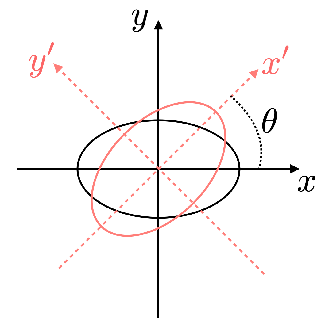
Second order moments: Here we discuss the second order moment of an ellipse with constance surface brightness \(\mu\) (not in magnitude). Assume we have correct the coordinate origin to the center of this ellipse. The the horizontal aligned ellipse (black one in the right figure), it’s straightforward to calculate its second order moments as: \[M_{2, 0} = \frac{1}{4}a^2,\ M_{0, 2} = \frac{1}{4}b^2,\ M_{1, 1} = 0.\] We already see that the second order moments contain information about the shape, size and orientation of an ellipse. Then we study a non-trivial case by rotating the ellipse by \(\theta\) (pink ellipse). We are very familiar with the coordinate transformation between \((x, y)\) and \((x', y')\), which is written as \[x’ = x\cos\theta - y\sin\theta,\ y’ = x\sin\theta + y\cos\theta.\] Plug in these transformation and express \(M_{2, 0}'\) using \(M_{2, 0},\ M_{0, 2},\ M_{1,1}\), also noticing the Jacobian of this transformation is unity, we have: \[M_{2, 0}’ = \frac{1}{4}(a^2\cos^2\theta + b^2\sin^2\theta),\] \[M_{0, 2}’ = \frac{1}{4}(a^2\sin^2\theta + b^2\cos^2\theta),\] \[M_{1, 1}’ = \frac{1}{4}(a^2 - b^2)\sin\theta\cos\theta.\] Then we can define a complex ellipticity which goes like \[\widetilde{e} = \frac{M_{2, 0}’ - M_{0, 2}’ + 2i M_{1, 1}’}{M_{2, 0}’ + M_{0, 2}’}.\] And it turns out to be \[\widetilde{e} = \frac{1-q^2}{1+q^2}(\cos 2\theta + i\sin 2\theta),\] where \(q\) is the axis ratio \(b/a\), and \((1-q^2) / (1+q^2) = e\) is the ellipticity of the ellipse. Thus \[\widetilde{e} = e_1 + i e_2 = e(\cos 2\theta + i\sin 2\theta).\] Hence we have many combinations to express the shape (ellipticity and position angle) and size: \((\theta, e)\), \((e_1, e_2)\), etc.
Higher order moments tell us the distortion and anisotropy of the image. Using higher order moments, we can estimate the PSF structure and how well does the PSF model behave.
For shape measurements based on moments, see this paper.

From Images to Catalogs

The signal of weak lensing is so weak that can be easily covered by all kinds of systematics. What observers need to do is to minimize these systematics.

PSF modeling

The effective PSF is composed of atmospheric PSF, optical PSF, pixel response difference, etc (P.S. Rachel Mandelbaum is one of the authors of GalSim). The optical PSF can be generally modeled and is easier compared to atmospheric PSF.

Why does PSF affect weak lensing? Weak lensing measures the shapes of (faint) galaxies, PSF can make the galaxy itself more circular, make the shape of outskirts irregular (due to PSF anisotropy), and also make deblending very hard.
How to measure PSF? Generally we measure the profiles of stars in the field as PSF models, then interpolate (using regular polynomials or Chebyshev polynomials) these models to other positions where we concern. But interpolation often make sense only on single CCD level. PSF model behaves bad on the edges of CCDs (but can use dithering and PCA interpolation to mitigate).
PSF estimated by stars might not be accurate for galaxies. PSF actually depends on the SED of objects, but stars and galaxies have different SEDs. This effect is especially severe for very-wide-band surveys (Euclid). Also the PSF estimated by bright stars are not suitable for galaxies (even not suitable for bright galaxies).

Detector Systematics

Brighter-fatter effect. The electric field sourced by charges accumulated within a pixel can deflect the later coming electrons away, and the consequence is to enlarge the boundaries of the object. So we don’t measure PSF from bright stars. Also saturation is an additional factor.
Some other defects of detectors can also considered as systematics. The difference of pixel sized among all pixels results in astrometric and photometric errors. The responding of pixels may also correlated with galaxy shape and position. In the next generation near infrared survey (WFIRST), we need to mitigate systematics related to NIR detector defects (they are not CCDs).

Deblending

The final goal of deblending is to separate the lights from blended objects, and then measure the shapes. There are generally two kinds of blending. One is called ‘recognized blending’, in which you/algorithms can clearly detect two or more objects. The other is called ‘unrecognized blending’, in which you cannot tell things apart by eyes/algorithms easily.

Deblending allow us to use larger sample, otherwise we have to exclude (e.g. CFHTLenS) those blended sources (which account for 50% in HSC).
Deblending allow us to give sources better photo-\(z\). If two galaxies with different SED/redshift blend together and we consider them as one source, then the photo-\(z\) can go weird.

Now there are many deblending algorithms, some of them take the advantages of the state-of-art machine learning and deep learning techniques. It’s easier to distinguish objects by combining multi-band images than just looking at single band. Peter Melchoir write the deblending package scarlet based on multi-band images. And guys at UCSC also try to deblend images using GAN (Generative Adversarial Networks) 🔗.

Image Combination

: Nyquist Sampling Rate

We all know that longer exposure time gives better S/N image. So we stack single-CCD images together to get deeper detections. The stacked image is usually called ‘coadd’. But ‘coadd’ is not only for getting deeper (which is usually the case for ground-based telescopes). The pixel sizes of space-based telescopes are mostly quite large, so the image is under-sampled.

What is Nyquist sample rate? For a sinusoidal time series with frequency \(f\), if the sampling rate (frequency) is smaller than \(2f\), you cannot get the correct frequency from the sampled data. Also if the sampling rate is below \(2f\), you cannot distinguish between two frequencies since they behave similar under this sampling rate.

This paper 🔗 describes the obstacle of space telescopes whose pixel sizes are limited by some reasons. If the pixel size is small and also large FOV is wanted, then you will need more CCDs, thus a heavier satellite will be launched with much more money. For Euclid, the pixel size is larger than the Nyquist pixel size (which is determined by the resolution \(\lambda/D\)), thus the images are under-sampled. But this can be mitigated by dithering, which is also image combination.

For ground-based telescopes, there are basically two ways of using coadds. One is to do all science (measure flux, shape and estimate PSF) based on coadds. The other is to estimate PSF on the appropriate weighted combination of single-exposure PSF, but use coadds to measure properties of galaxies. This way doesn’t waste the frame with best seeing.

“Representing the galaxy and PSF models as sums of Gaussians with different scale radii can drastically speed up the calculations.”

Other Aspects of Image Processing

Sky subtraction always affect everything. Errors in sky subtraction can cause coherent problems with object detection, photometry, and shear estimation near very bright objects—bright stars or collections of bright galaxies (e.g., in galaxy clusters).