

前2天有点事没能及时回复,不好意思。上面的讨论很好,总结起来, (1)这些ring galaxies 在SFR-mass图上到底主要是分布在GV(pipe3d的SFR)还是passive sequence(MPA的SFR)其实并不重要。Ring galaxies只是inside out过程中的一个phase,重要的是搞清楚导致ring形成(或者inside out quench)的物理机制,到底是由于AGN还是bar的作用
(2)当然,如果能限制一下这些ring galaxies在SFR-mass图上的位置还是很好的,特别是SFR(pipe3d)-SFR(mpa)的图上可以看出,ring galaxies的分布和其他galaxies比,是由systematic difference的。建议嘉轩用不同的SFR indicator看看,比如UV-based SFR和WISE的。嘉轩可以问问程鹏和可欣哪里去找这些SFRs
(3)嘉轩最后发的那个折线图,x轴换成sSFR,估计那些不同stellar mass的线就基本叠加在一起了。然后画这种折线图用moving average画(不会的画可以问问程鹏)。
(4)第一步,我们是要搞清楚ring galaxies里的AGN和bar的情况。其实,ring galaxies只是galaxies,主要是massive galaxies由inside out quench的过程中的有显著特征(出现ring)的一个phase,下一步是要搞清楚处于不同phase(above MS,on MS, GV, passive)的galaxies中AGN和bar的情况。其实就是详细比较程鹏那个AGN fraction-sSFR和bar fraction-sSFR的2条线的相互关系。
(5)嘉轩提到的ring galaxies样本里有7个ellipticals,这个你可以把ID告诉可欣,可欣在MaNGA的数据里快速看看这几个galaxy有啥显著特点。如果有的话,就可以单独写篇letter来分析下。程程和程鹏的结果发现,star forming ellipticals的quench也是inside out的,但数目相比disk的少很多。如果嘉轩这几个确定是出现了ring的ellipticals(应该就是inside out的结果),那就非常好了,可以细致分析下这几个galaxy的其它物理量。
cube=fits.open(‘XXXXX’)
cube[‘FLUX’] (还有WAVE, IVAR, MASK
cd 到指定位置。
rsync -avz rsync://data.sdss.org/dr14/manga/spectro/pipe3d/v2_1_2/2.1.2/images ./
MaNGA uses integral field unit (IFU) spectroscopy to measure spectra for hundreds of points within each galaxy.
MaNGA will provide two-dimensional maps of stellar velocity and velocity dispersion, mean stellar age and star formation history, stellar metallicity, element abundance ratio, stellar mass surface density, ionized gas velocity, ionized gas metallicity, star formation rate and dust extinction for a statistically powerful sample.
redshift z~0.03
selection cuts applied only to redshift, i-band luminosity, and for a subset of galaxies, NUV-r color.
Roughly flat stellar mass distribution with M > 10^9 M☉
IFU size from 19,37,61,91,127 fibers, diameters from 12″ to 32″
Data Reduction Pipeline (DRP)
objra, objdec, ifuglon, ifuglat, ifura, ifudec, airmsmed, seemed, g/r/i/zfwhm, zmin, zmax, szmin, szmax, ezmin, ezmax
nsa_z:红移
nsa_elpetro_absmag(Absolute magnitude in rest-frame SDSS ?-band, from elliptical Petrosian fluxes (NSA)),
nsa_elpetro_flux(Elliptical SDSS-style Petrosian flux in SDSS -?band (using r-band aperture) (NSA)),
nsa_sersic_absmag(Absolute magnitude in rest-frame SDSS ?-band, from Sersic fluxes (NSA))
nsa_sersic_flux(Two-dimensional, single-component Sersic fit flux in SDSS ?-band (fit using r-band structural parameters) (NSA))
nsa_sersic_th50: 50% light radius of two-dimensional, single-component Sersic fit to r-band (NSA)
nsa_sersic_phi: Angle (E of N) of major axis in two-dimensional, single-component Sersic fit in r-band (NSA)
nsa_sersic_ba: Axis ratio b/a from two-dimensional, single-component Sersic fit in r-band (NSA)
nsa_sersic_n: Sersic index from two-dimensional, single-component Sersic fit in r-band (NSA)
nsa_petro_flux_r: Azimuthally-averaged SDSS-style Petrosian flux in SDSS r-band (using r-band aperture) (NSA)
nsa_petro_th50: Azimuthally averaged SDSS-style Petrosian 50% light radius (derived from r band) (NSA)
nsa_extinction_r: Galactic extinction from Schlegel, Finkbeiner, and Davis (1997), in SDSS r-band (NSA)
In these catalogs, each galaxy has a unique MaNGA-ID. Each galaxy has a unique MaNGA-ID, but a galaxy may have multiple PLATE-IFUDESIGN designations if it has been observed multiple times.
row-stacked spectra (RSS) and datacubes (CUBE) files that are sampled either linearly (LIN) or log-linearly (LOG) in wavelength
DAP:These science-grade data cubes are then processed by the MaNGA Data Analysis Pipeline (DAP), which measures the shape and location of various spectral features, fits stellar population models, and performs a variety of other analyses necessary to derive astrophysically meaningful quantities from the calibrated data cubes.
a LINEAR version with a wavelength step of 1.0 Angstroms per pixel, and a LOG version with a wavelength step of 1e-4 in units of log10(lambda/Angstroms) per pixel.
The RSS file contains all spectra acquired in each exposure in a single 2D array; for example, an RSS file for a 19-fiber bundle may contain 19(fibers)4(dither sets)3(exposures per dither)=228 spectra, each with the same number of spectral pixels.
The CUBE file uses the RSS spectra to construct a uniformly sampled datacube, a 3D array with WCS coordinates (RA, DEC, λ); the spatial sampling is set to 0.5″ spaxels, but the spatial point-spread function (PSF) in the datacube is roughly 2.5″ at FWHM.
when reforming the raw spectra to a useful diagram, drp uses either LINEAR wavelength coordinate or LOG wavelength coordinate.
The difficulty with the CUBE data is due to the significant covariance between adjacent spaxels. Each spaxel is approximately 20% of the FWHM of the spatial PSF meaning that a single fiber contributes to many spaxels. Analysis of the datacube should then account for this spatial covariance; i.e., one should not treat the datacube as containing independent spectra.
The typical site seeing has a full width at half maximum (FWHM) of 1.5″. Our hexagonal-formatted fiber bundles are made from 2″-core-diameter fibers with 0.5″ gaps between adjacent fiber cores. So MaNGA use dithering. The three “dither” positions form a equilateral triangle with 1.44″ on a side.
Data in CUBE is a regular 0.5 arcsecond grid (in r.a. and dec., these two directions).
Python
It is possible to obtain a list of all the observed plates from the drpall file, as well as select plates that contain certain targets in which you are interested. Using Astropy and Numpy to obtain a list of all reduced plates, you can do
from astropy.table import Table
import numpy as np
drpall = Table.read('drpall-v2_1_2.fits')
plates = np.unique(drpall['plate'])
At this point you may want to reject plates without galaxy targets, for instance:
targets = drpall[np.where((drpall[‘mngtarg1'] > 0) | (drpall['mngtarg3'] > 0))]
plates = np.unique(drpall['plate'])
If you are interested in finding all plates that contain ancillary targets for a specific program, you can use the manga_target3 column (see more about bitmasks). For instance, the bit for the Milky Way analogues program is 13. To get the plates for the two observed targets in DR14, we do
targets = drpall[np.where(drpall['mngtarg3'] & 1<<13)]
plates = np.unique(targets['plate'])
Apply bitmasks and select region around Hαα:
do_not_use = (mask & 2**10) != 0
flux_m = np.ma.array(flux, mask=do_not_use)

redshift = 0.0402719
ind_wave = np.where((wave / (1 + redshift) > 6550) & (wave / (1 + redshift) < 6680))[0]
halpha = flux_m[:, :, ind_wave].sum(axis=2)
im = halpha.T

# Convert from array indices to arcsec relative to IFU center
dx = flux_header['CD1_1'] * 3600.  # deg to arcsec
dy = flux_header['CD2_2'] * 3600.  # deg to arcsec
x_extent = (np.array([0., im.shape[0]]) - (im.shape[0] - x_center)) * dx * (-1)
y_extent = (np.array([0., im.shape[1]]) - (im.shape[1] - y_center)) * dy
extent = [x_extent[0], x_extent[1], y_extent[0], y_extent[1]]
Note: How to find the redshift of a galaxy from the drpall file
Generate plot:
plt.imshow(im, extent=extent, cmap=cm.YlGnBu_r, vmin=0.1, vmax=100, origin='lower', interpolation='none')
plt.colorbar(label=flux_header['BUNIT'])
plt.xlabel('arcsec')
plt.ylabel('arcsec')
The Press–Schechter formalism predicts that the number of objects with mass between and is:
where is the mean (baryonic and dark) matter density of the universe, is the index of the power spectrum of the fluctuations in the early universe , andis a critical mass above which structures will form.
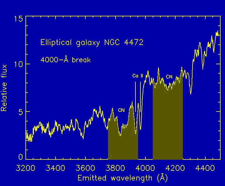
Literature and Galaxy Zoo talked about break. Briefly speaking, break is the ratio between the average flux density in and in . We can see from Fig.1, the ratio of average flux density in this two area can be calculated easily.
And break can be a proxy for stellar age of one galaxy, as Fig.2 shows.
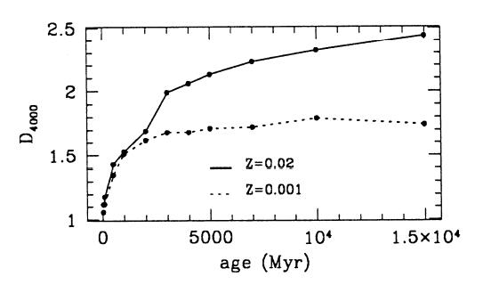
As we can see, ratio is proportional to the stellar age in a galaxy.